Module 1: Getting Started with GLM
Module Resources
Download the GLM files for this module by clicking the download button in the tool bar .
Setting up GLM
Running GLM on MacOS
- Open the Terminal application on your Mac
- Use the
cd(change directory) command to navigate to the Kinneret97 folder - In Finder, go to the macGLM folder and right-click on the glm app, select Show Package Contents
- Enter the Contents folder then the MacOS folder, and locate the glm executable file
- Back in terminal, enter the file path for this executable file - you can do this by dragging/dropping the file into the terminal
- Leave a space after the file path and type
--xdisp - Press Enter and the model will open
Running GLM on Windows
On Windows, the model can be run using a batch-file glm.bat, which you can double click from in the Kinneret97 directory. The .bat file calls the GLM model from the current working directory.
If the model is not opening make sure you’re not working in a network directory (e.g. OneDrive) and the file path to the glm.bat file has zero spaces in it.
Anatomy of a Simulation

Once the model has run, you can inspect the results. There are three ways to look at the output:
- Via the time-depth contour plots that appear during the run (configured via
plots.nml) - Further information on the daily water and energy balance is in the output file
lake.csv - Time series values of selected state variables (e.g. temperature, salinity, etc…) can be requested for a specific depth (depth above bottom) – this is setup in
&outputs(eg.WQ_5.csv)
Exercise: Lake-scale Water & Heat Balance
The simulation in the Kinneret97 directory is an example 40m deep, monomictic lake that is used to supply drinking water and support an active fishery.
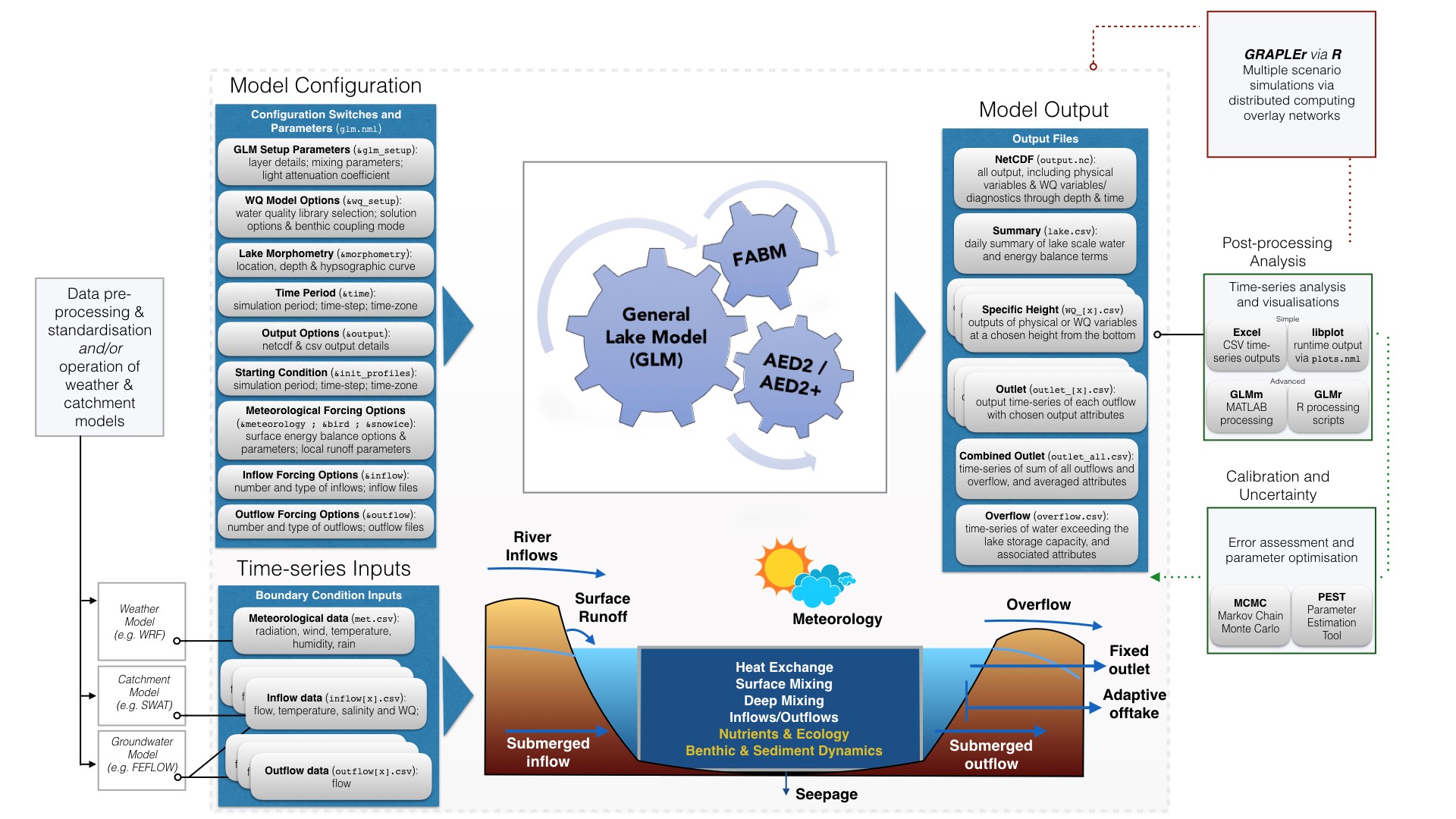
Before running the model, open the file glm3.nml in a text editor and inspect the model setup etc. This file is the main configuration file that drives the model. The file glm3.nml has several key sections in it related to the model domain and parameters, the sources of boundary condition data, and details of outputs. Scan the parameters, e.g. number of layers, light extinction coefficient, mixing coefficient etc.
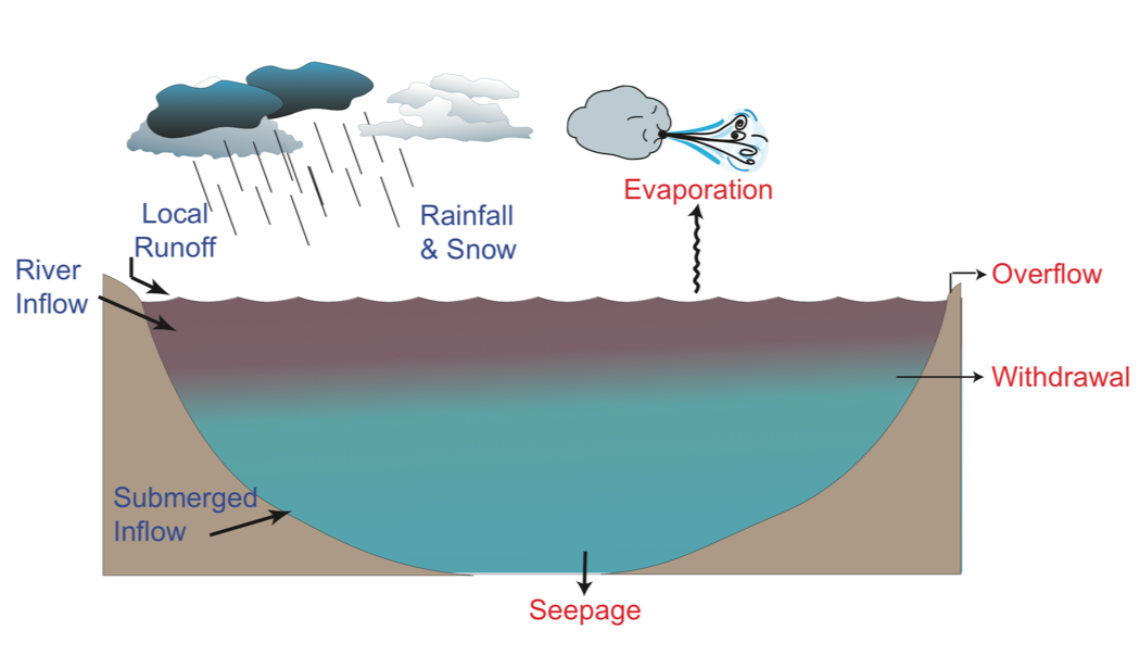
- Draw a schematic picture of the lake, the relevant boundary conditions (both related to water fluxes and energy fluxes).
- Identify and open the boundary condition input files - these are csv files containing time-series of meteorological information, and inflow and outflow volumes. These files can be opened in Excel or a text-editor. Find where these files are called from within
glm3.nml. - Plot the lake water balance – volume, water level and fluxes including inflows, outflows, rainfall and evaporation (refer to columns in
lake.csv, and copy the appropriate data into your own excel spreadsheet).

Figure 1: Schematic diagram of water balance components.
- Plot the surface heat fluxes such as shortwave, longwave, sensible heat latent heat (refer to columns in
lake.csv).
](images/09-module8/picture3.png)
Figure 2: Schematic diagram of surface heat fluxes impacting lake water temperature. For a description of the heat flux terms refer to the GLM paper