Week 6 (now week 5!) - Helena River data analysis
Learning Objectives
The practical activity for this week is designed to consolidate our knowledge of groundwater and surface water interactions, in the context of the Helena River site data-set (collected as part of Week 5 field visit).
This assessment will require students to understand how hydrologic monitoring can inform conceptual models of ecosystems, and how this can underpin solutions to management challenges.
The data set that you will work on is part of a long-term research investigation being undertaken with the WA Department of Biodiversity, Conservation and Attractions (DBCA) and UWA. The broader goal of this research is to understand the drivers of decline of E. rudis in relation to the changing hydrology regime at the Guildford floodplains at the terminus of Helena River.
At the completion of this activity, students will prepare an assessment that will demonstrate their ability to:
analyse and interpret measured hydrological data
develop a conceptual hydrological model
effectively communicate their understanding of a hydrological system through a written report
synthesize the information to make effective recommendations for managers.
The specific requirements of this assessment are located at the end of this page.
Our task
Our job when visiting this site is to use available data to us in order to delineate the hydrologic pathways (surface and sub-surface) that determine the distribution of water and salt in this floodplain ecosystem.
Changing salinity within river systems can cause shifts in floodplain vegetation which arise because of river water interaction with the floodplain. Depending on the salinity increase and the salt tolerance of the floodplain tree species, this can cause shifts in community structure. Eucalyptus rudis is important species that has a natural range along the Swan river and its tributaries. This species has been reported to be in decline for over 15 years along the Swan river (Clay & Majer 2001), and more recently along one of the tributaries of the Swan river: the Guildford floodplains of the Helena river (Dundas 2011). It is currently unknown the exact role of water availability and salinity in the observed decline, and alternate hypothesis related to tree pathogens (e.g. Phytophthora) are also considered to be drivers of decline You will use this information to develop a hydrological conceptual model of this site and develop a report that describes the context of the investigation and summarise the findings and observations as suitable for a reader such as the City of Swan Environmental Management team.
After your analysis you should be able to:
- Identify the surface water flow regime - where and when does surface water pond or flow
- Articulate the key features of the groundwater system - water level trends, groundwater flow directions, and surface water - groundwater interaction areas
- Assess the distribution of salinity in groundwater wells (piezometers) and surface water
- Conceptualise the hydrologic processes influencing salt movement and accumulation across the site
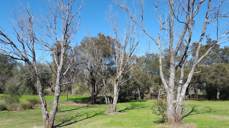
- Identify the distressed and dead trees at the site and articulate possible links between the hydroloigcal system and declining health of E. Rudis
The data you need for the assessment is a mix of previously collected data, and new data that is collected during the ENVT2251 field visit. The existing data is in the file Helena Data Combined.xlsx.
1. Investigating the site and vegetation change
There are now a range of spatial data products that have been generated from aerial imagery and remote sensing methods that we can use to help understand hydrological processes. One of these products is Nearmap, which allows us to access aerial imagery to investigate the changes in vegetation (and surface water distribution) over time.
Nearmap can be accessed at: http://maps.au.nearmap.com (login via UWA library Onesearch - see this webpage for details). Once you have successfully logged into Nearmap you can find the study site by searching for Guildford and then identifying the confluence of the Helena and Swan Rivers.
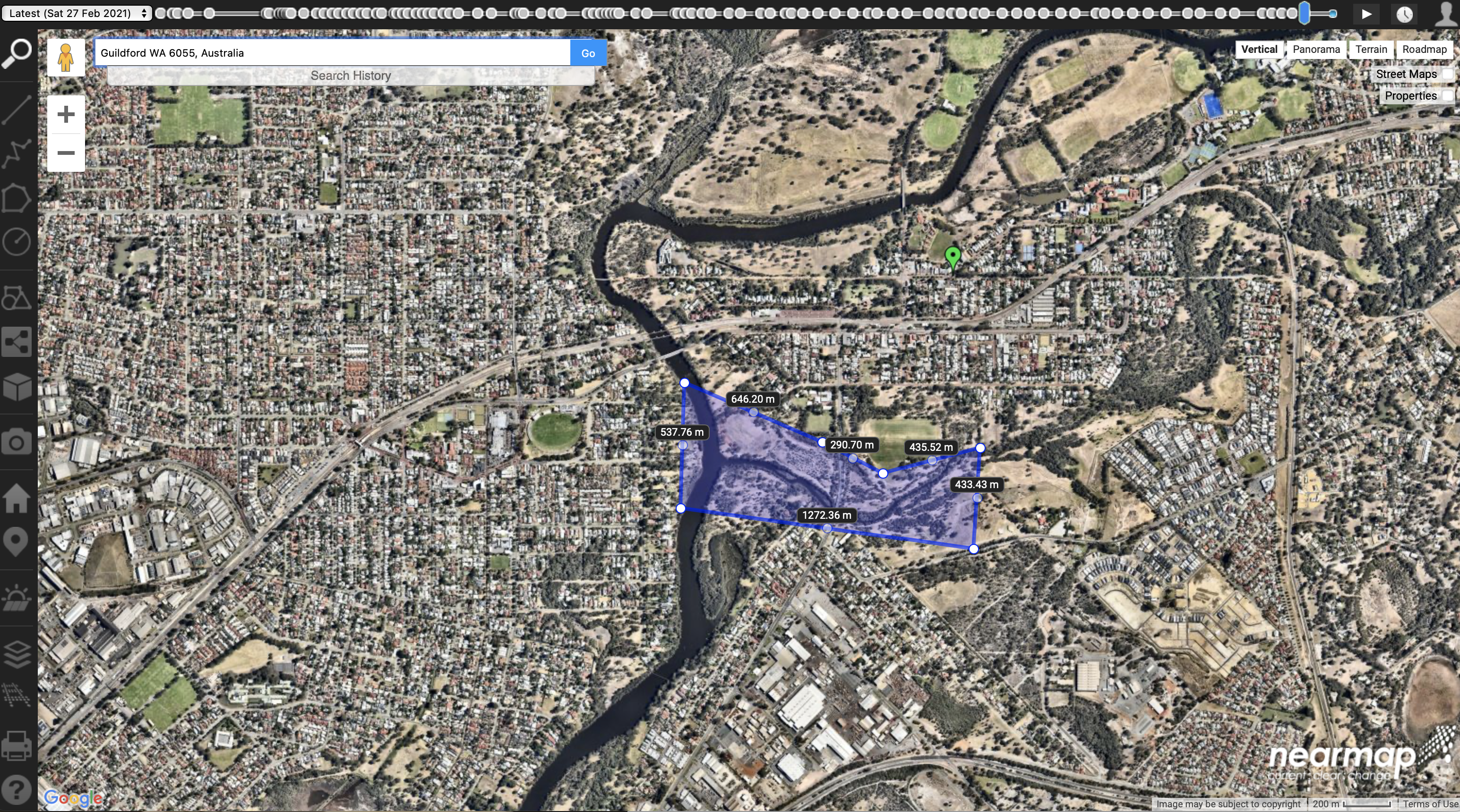
Figure 60: In Nearmap you can search for Guildford (green marker) to help you locate the study site at the confluence of the Helena and Swan Rivers (Blue shded area)
The City of Swan has identified our focus site on the Helena River near Guildford as an area of concern due to the decline of Eucalyptus rudis. This tree, termed the ‘flooded gum’ plays a vital role in the riparian ecosystem. Riparian woodland species are important filters that reduce nutrient transfers from the land into the river, which is a significant issue in the Swan river and its tributaries (excessive nutrients have historically resulted in noxious algal blooms). There is therefore a need to better understand what drives decline and if projected drying conditions brought about by climate change will make the pressures worse.
Zoom in so that you can see the vegetation canopy clearly and then use the time bar at the top to look at changes over time (play button will scroll through all available images, clock icon will split the screen so you can compare two different dates.
What seasonal changes can you see in the images?
How has the vegetation changed between the oldest and the most recent images (compare similar times of year)?
As you scroll through time does there seem to be a period of more rapid decline? Are there any periods of recovery?
The natural surface drainage of the site has been altered by artificial surface drainage channels.
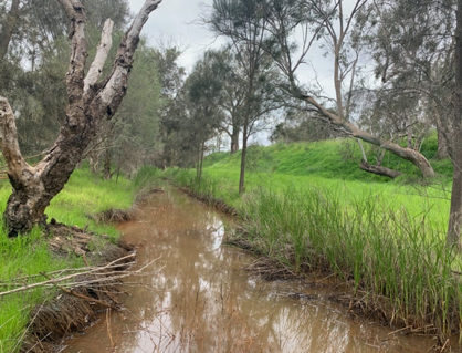
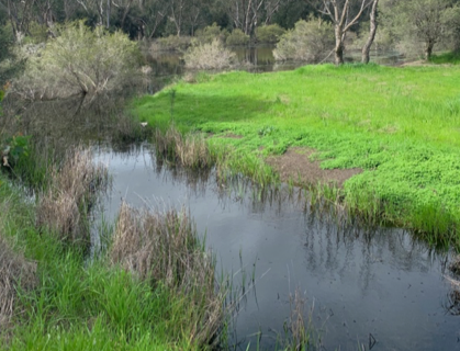
You can also see the distribution of surface water on the Nearmap imagery - compare what you see with the following mapping of surface water inundation at the site.
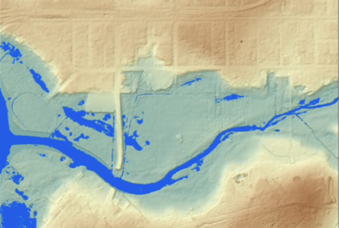
Figure 61: Example inundation pattern. Which way is the water flowing?
2. Time-series data for assessing water levels and salinity
You are provided with a spreadsheet that summarise the timeseries data collected by various agencies (e.g., UWA and DWER (via WIR)). This files includes numerous sheets with the following data notes :
GW Levels: This includes the UWA piezometer level data (converted into mAHD) for the main wells: HW1, HW2, and HW3. Bore 7 is also included which is denoted as Jeremy on the map.
GW Salinity: This has the UWA salinity measurements from inside the Piezometers. These data are in mS/cm.
Helena River: River Corrected data is the water level of Helena River under the nearby Traffic Bridge. So you can think of this as the water level at the river-end of the piezometer transect. “Poison Lease” (upstream in Helena River to the east of our site). It also has the discharge (Q) at this site, based on a rating curve.
Swan River: This has WIR data from the station MSB data as above, including the daily min and mix, showing the tidal amplitude of the Swan River over time. The “Vitox” Salinity data is from the WIR website for the nearby location which is just to the west of our site (on the other side of Kings Meadow Oval). This data indicates the river/estuary salinity and would be very similar to the salinity of the surface water in Helena River near our site also. Note its seasonality, compared to the groundwater.
2a. Groundwater levels and salinity
A series of monitoring wells have previously been installed at the site. The following LIDAR image shows the surface topography, with the locations of groundwater wells also indicated.
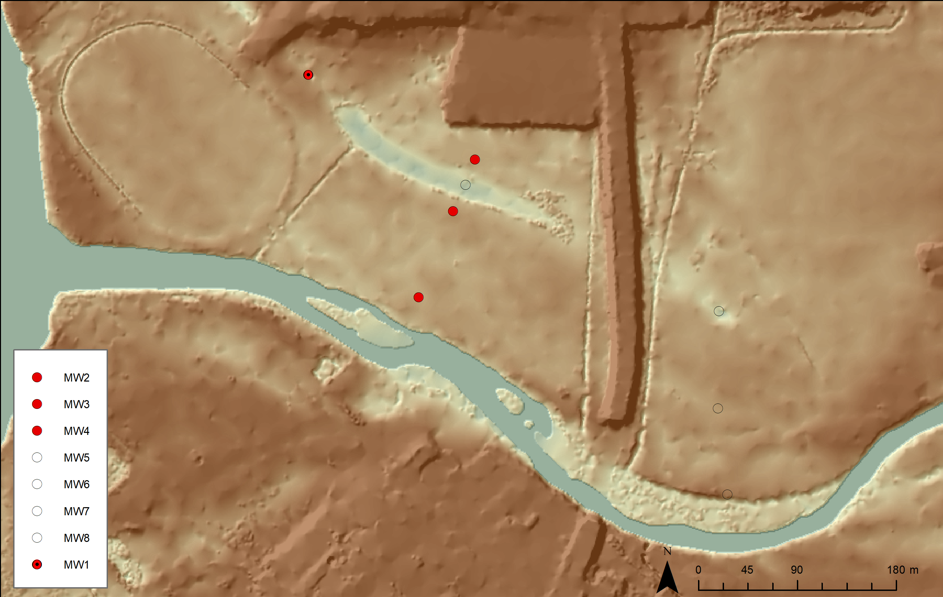
Figure 62: High-resolution LIDAR image of the surface topography of the Helena River study site in Guildford. The red-circles indicate groundwater observation wells.
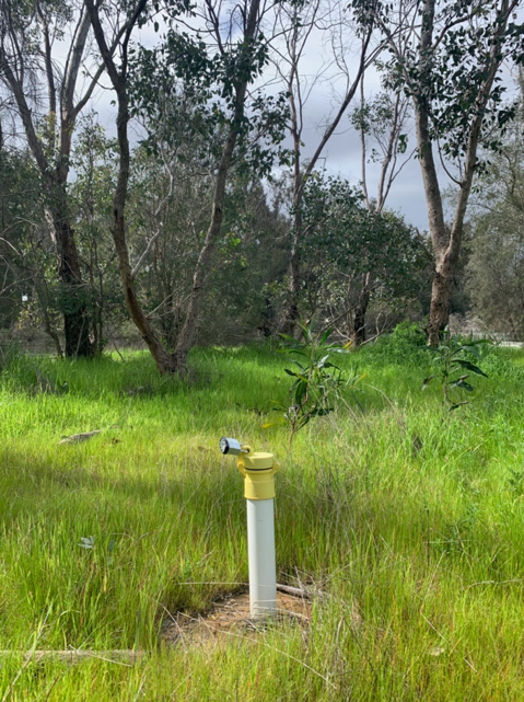
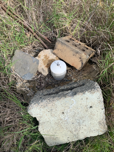
These groundwater monitoring wells are holes that have been drilled into the ground and lined with PVC pipes that has slots at the bottom to let the water in. All you can see from the land surface is the top of the PVC casing sticking up with a cap and sometimes a lock on it. If you want to use these wells for a scientific purpose you need to know the construction details. Firstly, where is the well (GPS coordinates) and what are the dimensions (depth and diameter) of the well? The well dimensions will determine the equipment you need to sample it. Secondly, across what depth range (and more importantly, elevation) is the screen interval (the area where slots are present)? This is the actual elevation of your groundwate pressure measurement; it’s important that you know this so that you carn compare your measurement with existing data. Once you get to a well, the first thing to do is measure the depth to water - from this measurement you can work out the elevation of the watertable, and also how much water is sitting in the well (standing water). If you want to sample for salinity or hydrochemical properties, then as a rule of thumb you need to remove 3-times this volume of standing water from the well before you take the sample to ensure the sample is representative of the aquifer.
Remember, when working with groundwater data you need to be careful to distinguish between groundwater levels that are reported as a depth to water (from the ground level or top of casing) as opposed to groundwater levels the Australian Height Datum (AHD). If there are measured values of depth to water you need to convert these to elevations in m AHD so they can be compared with the prior data and WIR data. To do this we need to know the ground level elevation at the measurement point, in mAHD (or the elevation of the top of casing, if this was the origin for the measurement).
Raw data is often not perfect, so think of some ways to present the data. For example,a PIVOT table is useful to look at monthly values. When interpreting the data we would like to highlight seasonality, and also relative differences between sites.
2b. Comparing groundwater and surface water changes
Now we want to try to find a way to bring togteher the different data into a single plot to help our interpretation of the what is happening at the system. That is, we have surface water data, and some groundwater data from different sources, but it is nice for us to compare them with each other so we can understand the nature of surface-groundwater interaction.
2c. Preparing a transect plot
If we recall Darcy’s Law, it is teh hydraulic gradient that can inform us which way water will flow. For example, if the water levels in the piezometer are higher than the mean river level, then aquifer water will discharge into the river. To visualise this gradient, we can plot the slope in the water table. At this site, if we compare the water table transect in different seasons, we can see the direction of flow reverses in some months.
3. Mapping salinity (EC) in QGIS
Specifically, a goal of ours is to understand the variability in salinity in the focus site.
Surface water samples from across the site have previously been collected and analysed for electrical conductivity (EC), which is a measure of salinity. Let’s create a map to visualise the spatial variation in salinity across the study site. The following instructions take you through the steps to do this in QGIS, which can be downloaded here. If you are proficient in ArcGIS you can use that instead to create your map.
Let’s start by importing our EC point data. Go to Layer -> Add Layer -> Add Delimited Text Layer.
Under File name navigate to a csv file of the EC data
- Make sure under File Format ‘CSV’ is selected
- Under Geometry Definition set the X field to the Easting column of you EC data and the Y field to the Northing column
- Set the Geometry CRS to “EPSG:32750 - WGS84/UTM zone 50S”
- Click Add
Figure 63: Importing your EC data.

You’ll now see the point data added to your screen, however, we have no spatial context - let’s add a basemap.
Go to the QuickMapServices (QMS) button in the toolbar and browse/search for a basemap that you think would be appropriate (e.g. search “satellite” and browse the different satellite basemap providers).
Add one to the map.
Figure 64: The QMS buttons in the QGIS toolbar.
Now we have a basemap and our points - let’s change the symbology of the points to better communicate the variation in EC.
- Right click on the point data in the layer window and go Properties -> Symbology.
- Set the symbol type to Graduated and specifying the values to graduate by as our EC column.
- Now set the Method to Size, and the Mode to Natural Breaks (Jenks), click Classify.
Figure 65: Changing the symbology of our point data.
Now when you click Apply the point size is weighted to the EC. You can further refine your symbology by changing the point colours and size - think about how best to communicate variation in EC.
- Finally, create a map output by clicking the New Layout button in the toolbar. If you aren’t familiar with creating maps in QGIS work with one of your classmates who is, or read through the second half of this tutorial.
Figure 66: Example map from your QGIS output.
4. Conceptualising Surface-Groundwater interaction
Start by reading this report by UWA researchers to learn more about the history of scientific studies at this site and recent findings:
Now that you have an understanding of the previous studies at the site, and have plotted the available data, the next step is to develop your conceptual model of surface water - groundwater interaction. When trying to make sense of all this data from different locations and time periods some guiding questions can help focus your analyses:
How does salinity vary across the surface water sites? How does this relate to sources of water (Helena River, Stormwater from nearby suburbs, Swan estuary, Rain)
How does water level and salinity vary in the groundwater based on distance from the river? Are levels in the aquifer higher or lower than the (mean) river level? What about salinity?
Do these patterns in groundwater salinity change seasonally?
Which flow pathways drive the changes we see? Is water moving vertically or laterally? Consider how water levels in the piezometers vary relative to surface water. Think here Darcy’s Law and Hydraulic gradient.
5. Reccomendations
The degradation of freshwater systems by increasing salinity is a major challenge facing Western Australia. Salinisation of the Avon river, which enters the Upper Swan river at Walyunga National Park, arose due to poor land-management leading to secondary salinity in the inland wheatbelt catchments. Whilst secondary salinity is not an issue in the Swan Coastal Plain where our study site is, the salt loads from the Avon in addition to rising sea levels and decreasing rainfall trend have been driving changes in the seasonal movement of brackish estuarine water, with increasing penetration of the salt wedge further inland from the ocean (Huang et al. 2018).
Can you think about monitoring or other research that could now be undertaken to further understand the situation? For example:
Are the unsaturated zone (vadose zone) conditions adequate for the tree roots? i.e., is the water table depth deep enough to contain non-salty soil moisture for them, or must they rely on water from salty groundwater? Look here at areas in nearmap where tree loss has occurred.
What are the salinity tolerances reported for E. rudis, based on lab/field trials in the literature? How does data we collected compare to the sort of data where salinity is known to impact the species?
Submission
Your report should include:
Introduction [1 page maximum]
Background and context – why are we interested in this site?
Map of site – where specifically are we looking at?
Scope of the investigation – what is this report about?
Assessment methodology [1 page : be concise!]
Desktop assessment, data sources (historical and present) – UWA and external data/info that has been referred to. A table can be convenient to summarise, or a structured list.
Data analysis approach, as relevant – any processing or “higher” analysis that was done to the data to make the assessment possible.
Results and findings [~3 pages]
Map of surface water salinity
Time-series graphs of climate, water levels, flows and salinities (or EC)
Transect of water level and salinity data across the site
Conceptual model of surface and groundwater flow and salt pathways; consider all information in this, including past data and reports and nearmap imagery. Consider how summer may be different to winter!
Discussion and conclusions [<1 page]
Interpretation of the data presented in light of the observed tree-decline locations
Suggestions for improved monitoring and further investigations; dot-points OK here.
Your report will be assessed according to the marking rubric on LMS. Submissions not received by the due date will attract a late penalty.
References
Clay, R., Majer, J. (2001). Flooded Gum (Eucalyptus rudis) Decline in the Perth Metropolitan Area: A Preliminary Assessment.
Hipsey, M.R., Alilou, H., Bourke, S., Bunting, C., Busch, B.D., Job, M., Whitwell, C., and Zhai, S., (2020). Understanding and predicting riparian decline: Ecohydrology and hydro-climatological change in the Upper Swan estuary. The University of Western Australia, Perth, Australia. 51pp. .