Exercise 5 - Visualising groundwater
Learning Objectives
In this exercise you will investigate what controls the direction and rate of groundwater flow.
At the completion of this exercise students will be able to
have experience describing Darcy’s Law
calculate groundwater flow rates
describe the range of flow rates within natural groundwater systems and explain the key factors controlling these rates
identify patterns of groundwater flow and hydraulic head contours within groundwater systems
Groundwater flow rates
As a first step lets consider the flux law for groundwater flow. Groundwater flow is driven by the distribution of water pressure (hydraulic head, which has units of length) within the groundwater system. The flow of groundwater follows a flux law;
where \(q\) is the specific discharge (or Darcy Flux) with units of L T-1, \(Q\) is the volumetric flow rate (L3 T-1), \(A\) is the cross-sectional area through which the water flow (L2), and \(\frac{\Delta h}{ \Delta l}\) is the hydraulic gradient. This gradient is simply the change in water pressure (\(h_1-h_2\)) over a given distance (L/L, unitless). The key system property in this flux law is the hydraulic conductivity (\(K\)), which has units of L T-1. In natural groundwater systems the value of hydraulic conductivity can vary over 12 orders of magnitude. Even though this water flux \(q\) has units of L T-1, it’s not actually the velocity of the groundwater, because the water wasn’t flowing through the whole area, just the pore space. To correct for this and calculate the average velocity we need to use the area of the pore space (\(An\), where \(n\) is porosity), instead of the total area. This gives us:
where \(\bar{v}\) is the average linear velocity of the water flowing through the porous media.
Now that we know these simple equations let’s look at some experimental data from simple “Darcy tubes” that allow us to measure the relationships between rates of groundwater flow, hydraulic gradients and the hydraulic conductivity of the porous media that it flows through. This is how the idea of a “hydraulic conductivity” was first defined, empirically, and it was only decades later that the physical basis for hydraulic conductivity and Darcy’s Law was fully elucidated from first principles (see Hubbert 1940 for some light bedtime reading).
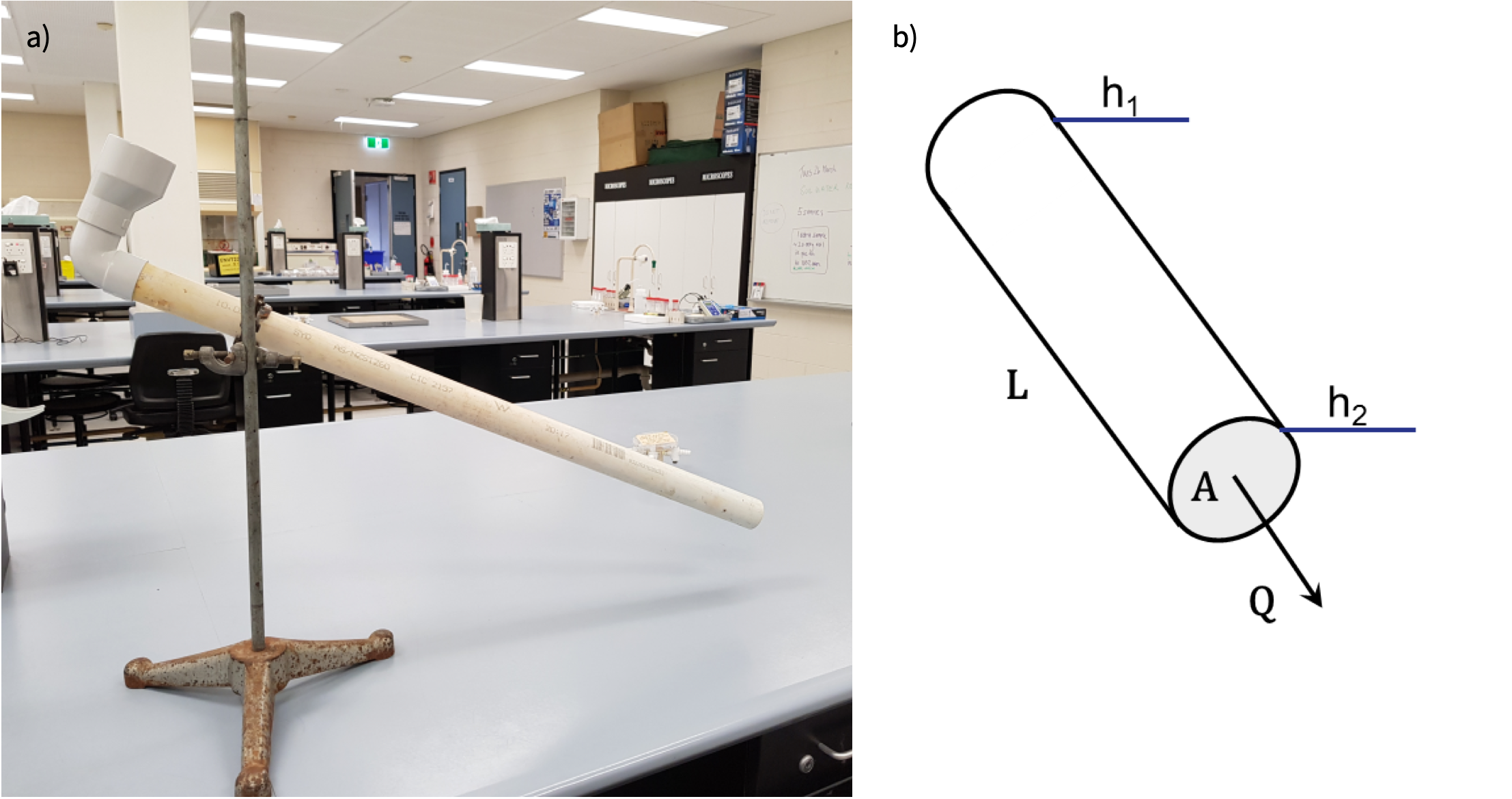
Figure 17: a) Photo of simple Darcy Tube and b) diagram showing terms in Darcy’s Law Equation
Let’s have a go at using this experimental setup to estimate the hydraulic conductivity of different sedimentary materials. To do this all we need to do is measure the flow rate through the tube for our chosen porous media. For each porous material, the slope determines the hydraulic gradient and we just need to measure the volume that flows out of the tube over a set time interval.
During this experiment;
the diameter of the tubes was 40 mm
the inlet at the top of the tube was 25 cm above the outlet at the bottom of the tube, and the lateral distance between the inlet and the outlet was 0.5 m
Over a period 24 hours 168 mL was collected from the tube filled with sand, 3.6 mL was collected from the tube filled with silty sand, and 814 mL of water was collected from the tube filled with gravel.
- Based on this information you can rearrange Eq (7) to calculate the hydraulic conductivity of each porous media.
Are you results consistent with the range of values for similar porous media in the literature? Could you measure the hydraulic conductivity of a clay sample using this experimental setup? What could you do to improve this experiment?
Using Darcy’s Law to calculate flow to a stream
Now we understand the concept of Darcy’s Law within a small-scale context, lets think about how we can apply it in the “real world”. The below diagram shows the flow in an aquifer towards a stream.
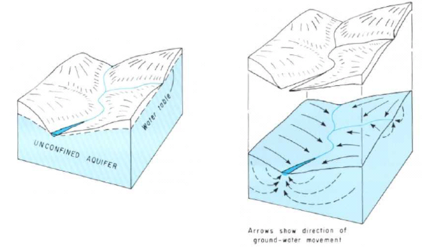
Figure 18: Water table and topography of a idealised hillslope
- Consider the diagram above. If the slope of the water table hydraulic gradient perpendicular to the stream is on average approximately 1/1000 (m/m), what is the Darcy flux, q, of groundwater towards the river? Use a hydraulic conductivity, K, of 1 m /day.
Groundwater flow concepts
We can trace the path of a “parcel” of water at any point in a groundwater system by creating a “flow net”. To do this we map the lines of “equipotential” (i.e., lines of constant head), like height contours on a topographic map, but instead of land height, its water height. Based on the gradient in water height (hydraulic gradient) we can work out the path that a parcel of water would take, as water will flow from high to low pressure.
Creating a flow net
Before we go further, lets check out this cool flow-net tool called “TopoDrive”. This is an online interactive tool that allows you to visulise groundwater flow nets!
.](images/exercise4/pictureY.png)
Figure 19: Creating a hillslope flow-net. For an overview, check out this youtube instruction video here.
- Create a hypothetical hillslope water table cross-section with the tool. Use the tool to show the water flow pathways. Make a note of your observations - is there anything unexpected? Depending on your flow-net you may be surprised that water does not always flow in a straight line!
One thing to note with flow-lines (or sometimes we call them streamlines), water flow paths must cross lines of equipotetnial at right-angles (i.e. perpendicular).
Interpreting a flow net
- Now look at the below image - a plan view of the water table contours around Perth. Given the sort of hydraulic conductivities estimated above, what would the range of linear velocity we could expect in a groundwater system like the Gnangara Mound? Use the following watertable map (taken from Davidson and Yu 2008, HG20) to estimate a hydraulic conductivity, and then calculate linear velocity using Eq (8). You will need to assume a porosity - look these up, or just use 0.25 (which is a good indicative value for back-of-the-envelope calculations in aquifer materials - why not in clays?). Note that it’s probably ok to assume a porosity value because the range of porosity is within one order of magnitude, whereas hydraulic conductivity will vary by multiple orders of magnitude, even within the same type of material, so this will be the larger source of uncertainty in your calculation.
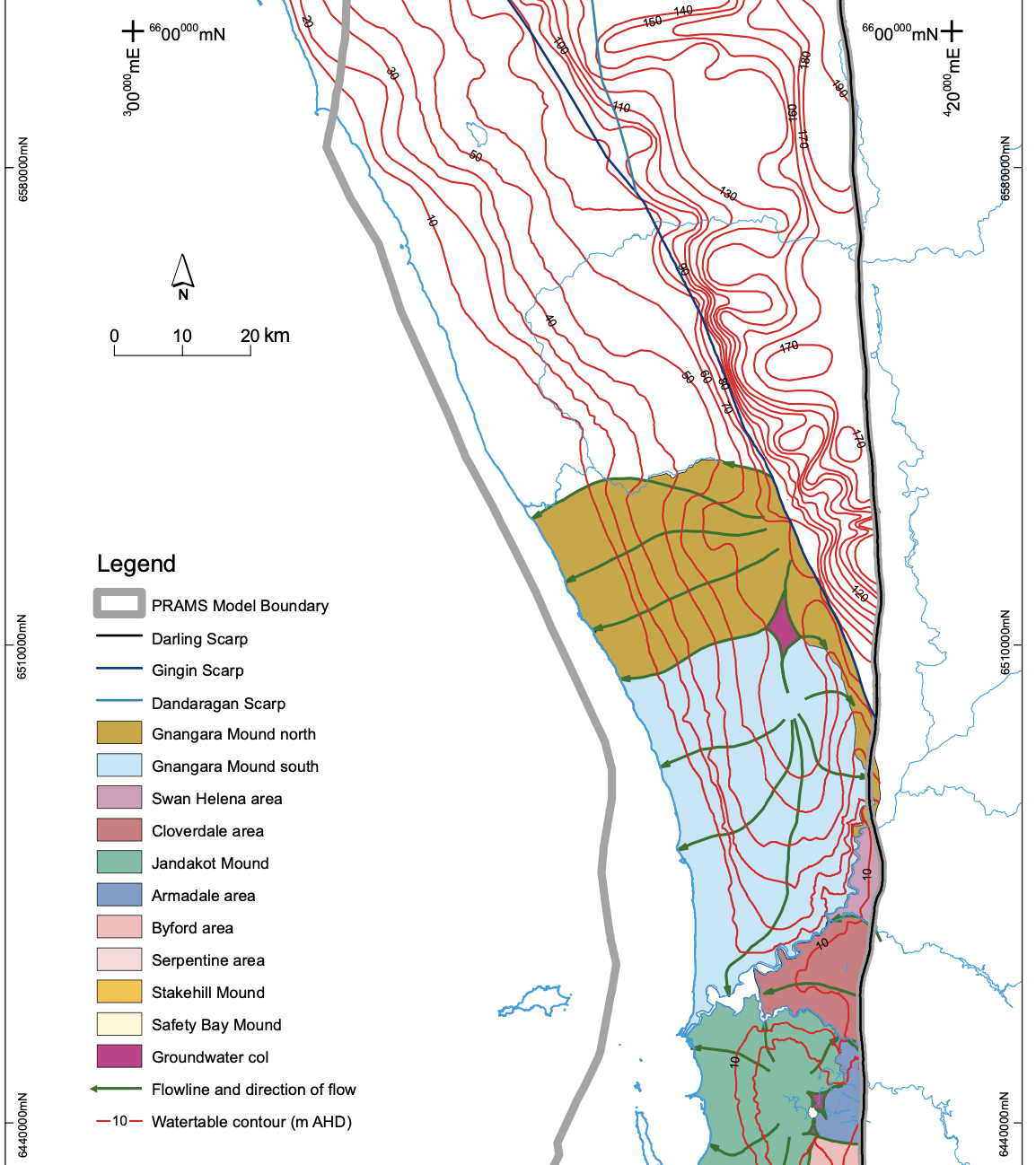
Figure 20: Section of a map of the watertable across Perth
Transmissivity
The transmissivity of an aquifer is the depth-integrated hydraulic conductivity, computed as:
- Using the diagram below, find the Transmissivity, T, of the system.
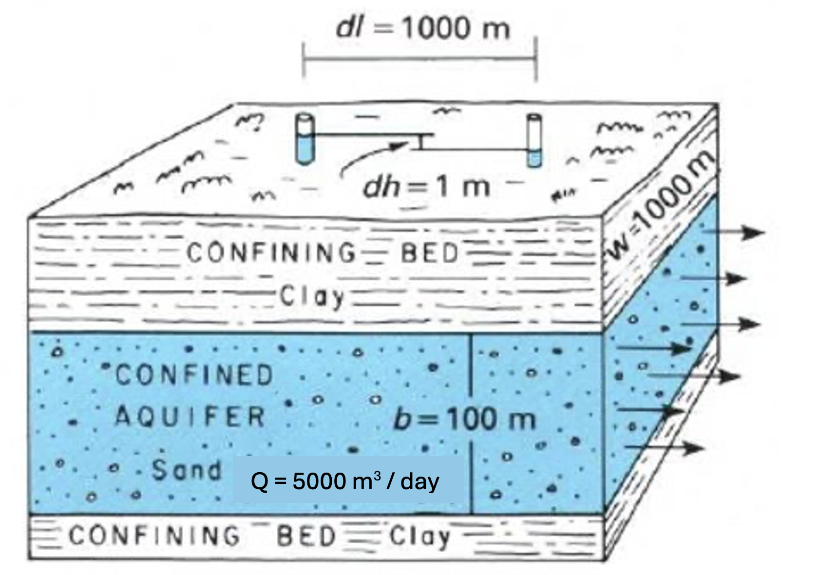
Figure 21: Annotated cross section of an aquifer
Example calculation of groundwater baseflow to a river
In this section is an example of how we can apply Darcy’s Law to work out how an aquifer is “working”, i.e., how much water it is conducting and entering the river as baseflow. Consider the following.
After a prolonged period without rain, the discharge of a river at a measuring station A is 10 m3/s and at a downstream station B it is 15 m3/s. The distance between A and B is 2 km.
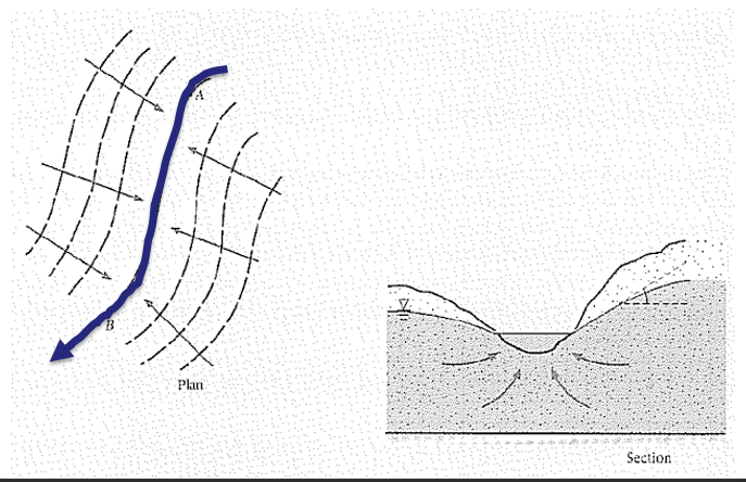
Figure 22: Plan and cross sectional view of a river valley
Between the stations, the river receives water from both sides, from an unconfined aquifer, and the equipotentials are assumed to be parallel to the river.
The slope of the water table (hydraulic gradient) on average is approximately 1/1000 (m/m).
- Based on this information, use Darcy’s Law to determine the transmissivity of the aquifer, in m2/s.
Start by drawing your own diagram and annotate with the information that you know.