Exercise 4 – Data synthesis
In the past two exercises we have processed rainfall data and streamflow data. This last exercise is to explore the shared data-set that spans sites across Western Australia, and to synthesise how this looks, in order to prepare our data analysis report.
Our overarching goal in prepaing our analysis is to summarise our findings on the nature of rainfall and runoff data we have explored across the state of Western Australia. Rainfall is influenced by a number of processes that operate on different space and time scales (see Figure 5). In Exercise 2, we examined rainfall trends and have explored how different modes of climate variability can explain patterns in annual rainfall. In Exercise 3, we have looked to see if we can find how strong the relationship is between (annual) rainfall and streamflow.
.](images/assessment2A/image1.png)
Figure 5: A guide to the timescales applicable to weather, climate variability and climate change Pacific Climate Futures.
So far, you have explored data from an individual site. But for our final data synthesis (and your assignment), we will make use of a larger number of sites across WA, to quantify the variability of rainfall and streamflow in space and time. Let’s start by making a summary of the spatial variability in rainfall.
Spatial patterns in rainfall
15) Inspect the results of everyone’s analysis in the shared data table(s). Are there statistically significant changes in rainfall? Which station(s) have a statistically significant slope? Are they consistent across WA? What may be causing the changes?
16) Take the information in tables and record the values onto a map of Western Australia.
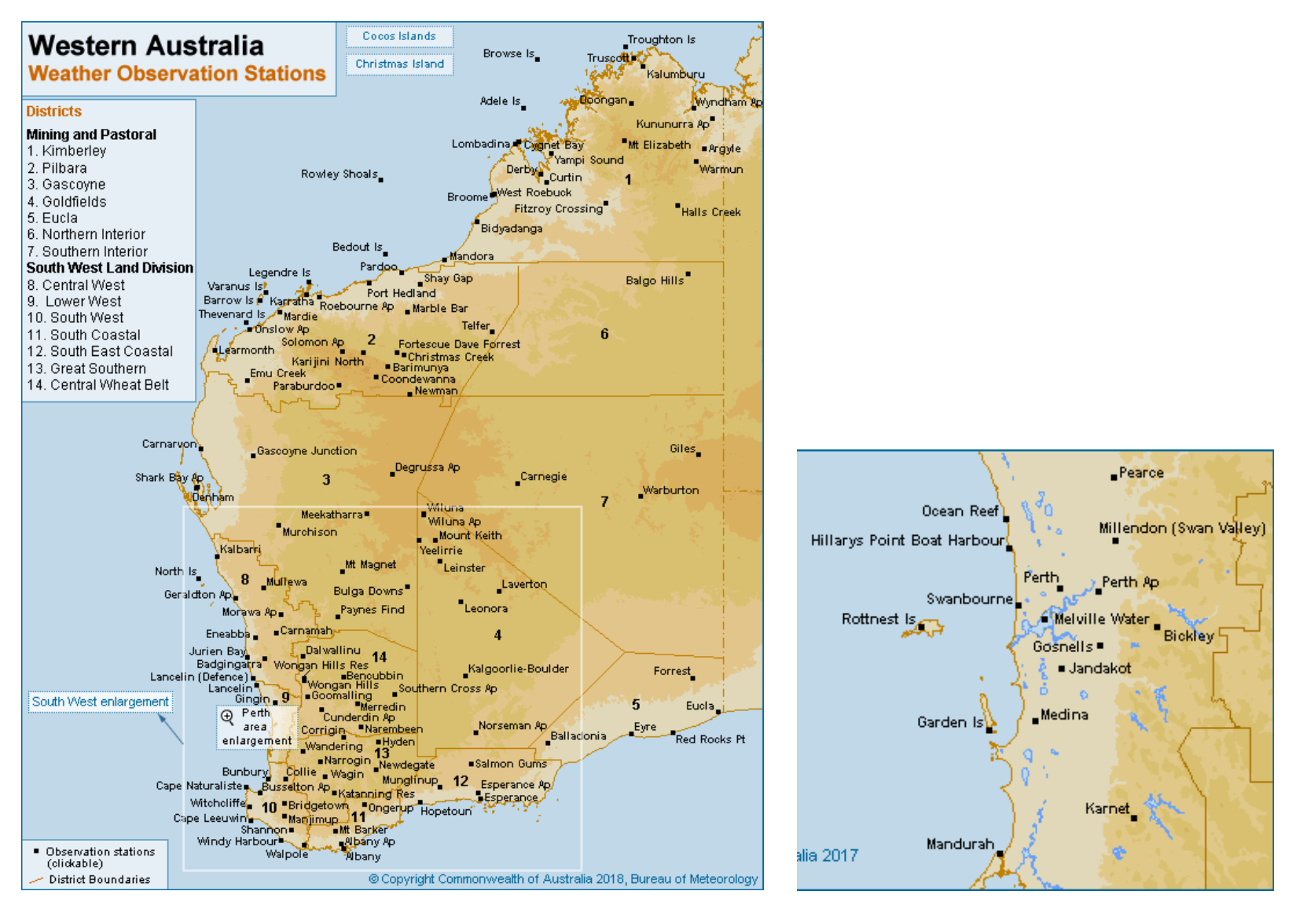
Let’s create a map to visualise the spatial variation in our selected rainfall properties across the state - let’s face it, maps are cooler than tables. The following instructions are to guide you through the steps to do this in QGIS, which can be downloaded here. If you are proficient in ArcGIS you can use that instead to create your map. Or if you prefer not to use GIS for this assignment, then you can also create a map in Google Earth and manually add some pins.
- In QGIS, start by adding a base-map. Go to the QuickMapServices (QMS) button in the toolbar and browse/search for a basemap that you think would be appropriate (e.g. search “satellite” and browse the different satellite basemap providers).
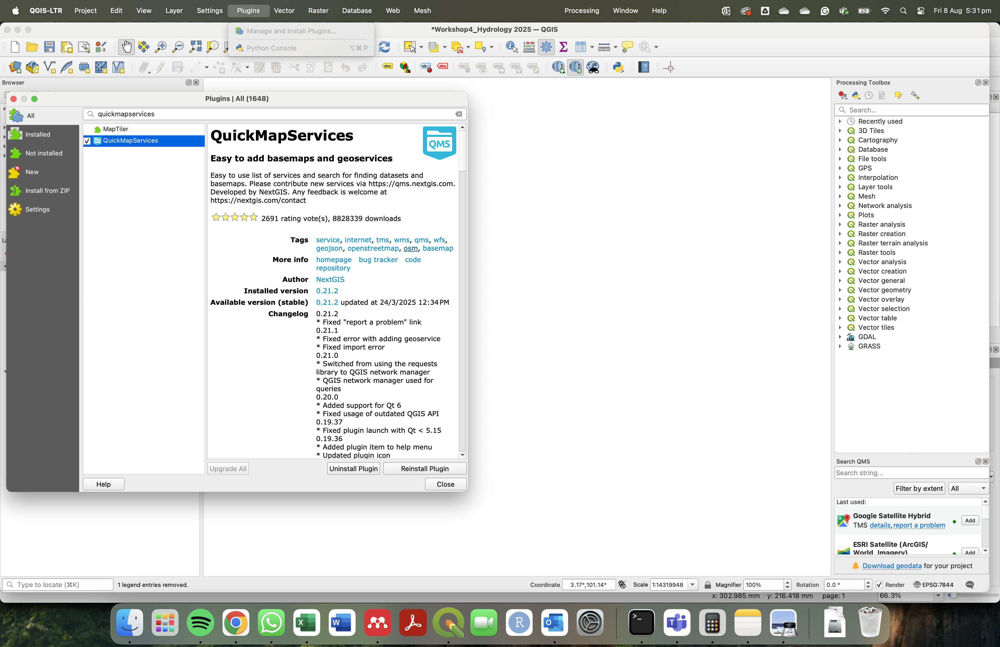
Figure 6: QuickMapServices.
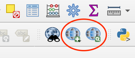
Figure 7: The QMS buttons in the QGIS toolbar.
- Click on the Search QMS icon. A search box will appear at the bottom right corner of your screen. Type satellite, select from one of the options. Click add.
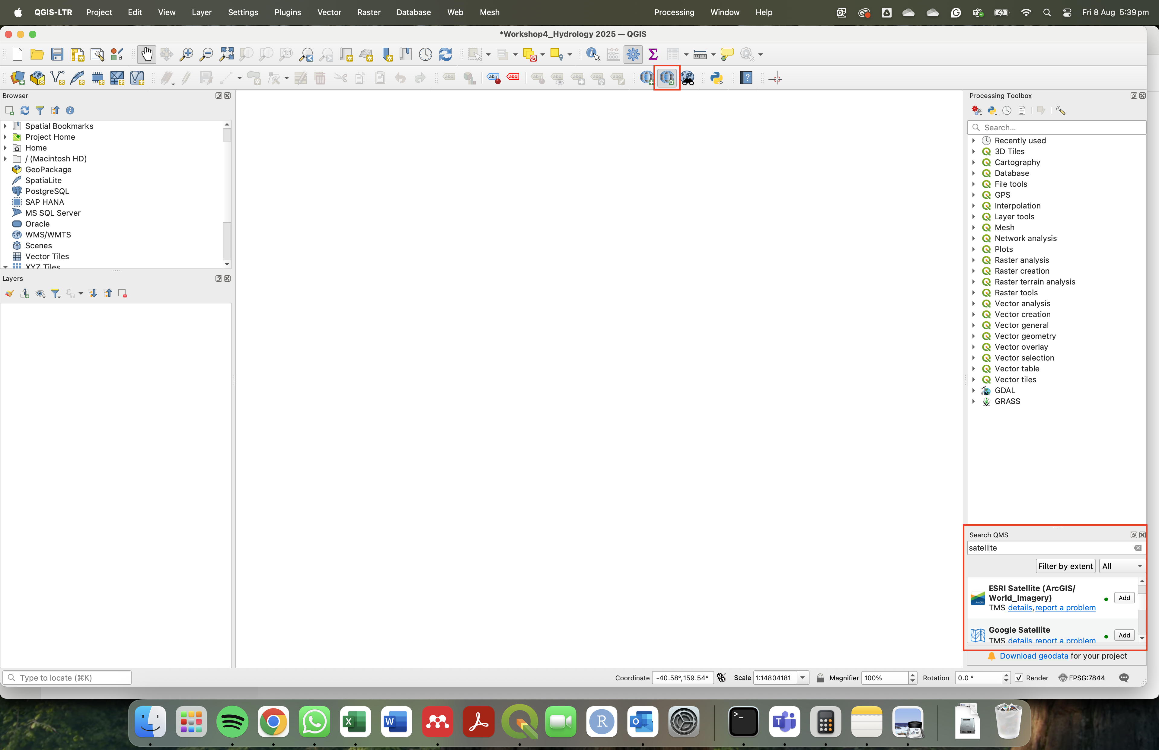
Figure 8: QMS search.

- To add the spreadsheet data, go to Layer -> Add Layer -> Add Delimited Text Layer.
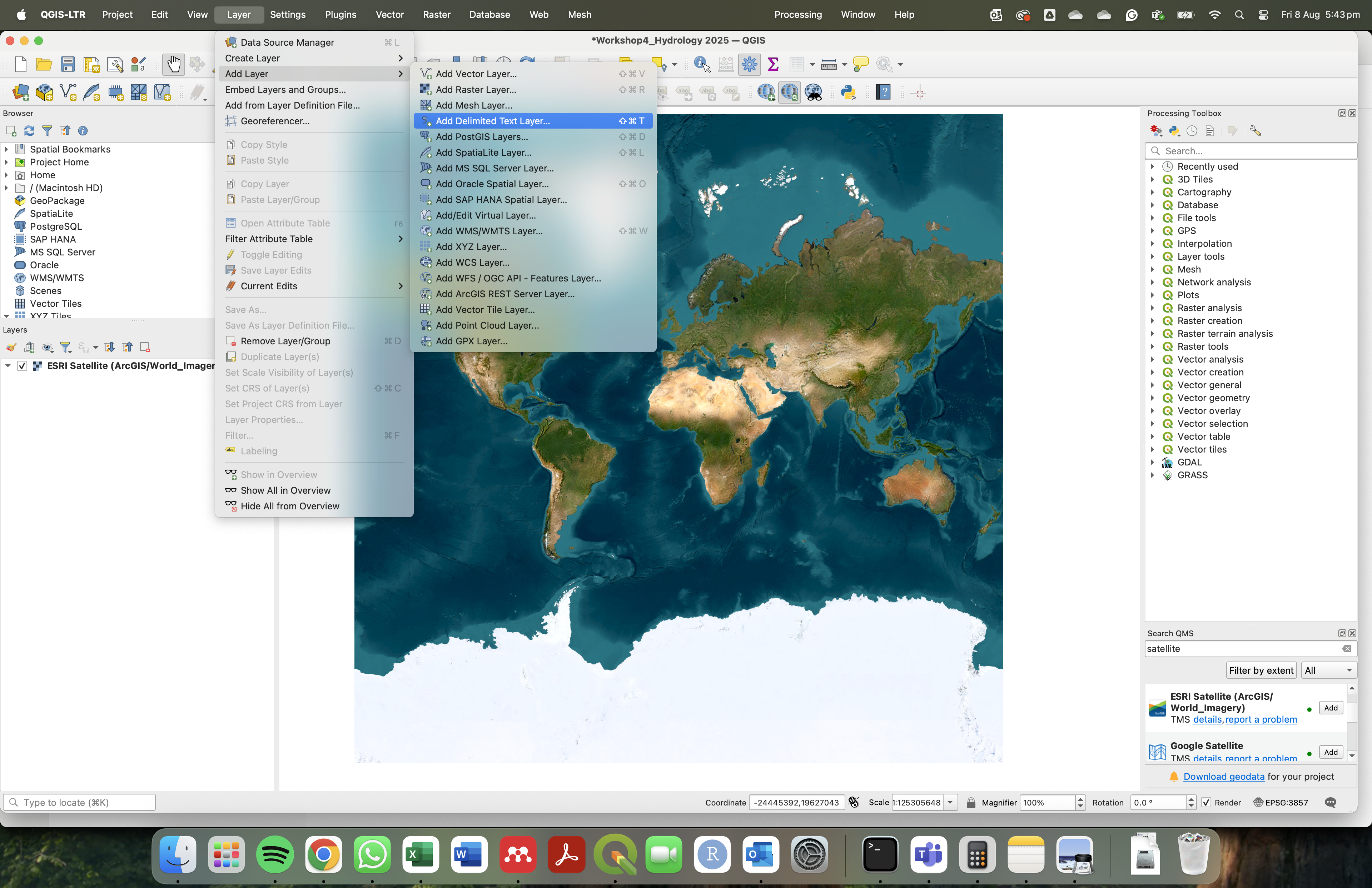
Figure 9: Finding data to add to the map.
Under File name navigate to the csv file which has the rainfall data
- Make sure under File Format ‘CSV’ is selected
- Under Geometry Definition set the X field to the Long column of your data and the Y field to the Lat column
- Make sure all the numerical values that have decimals are classified decimals in the Sample Data menu (check the table at the bottom)
- Now make sure you use the right Geometry CRS. In our case: “EPSG:7844 - GDA2020”.
- (If you don’t have the right CRS, click on the icon on the right side of the CRS field and search for GDA2020)
- Click Add
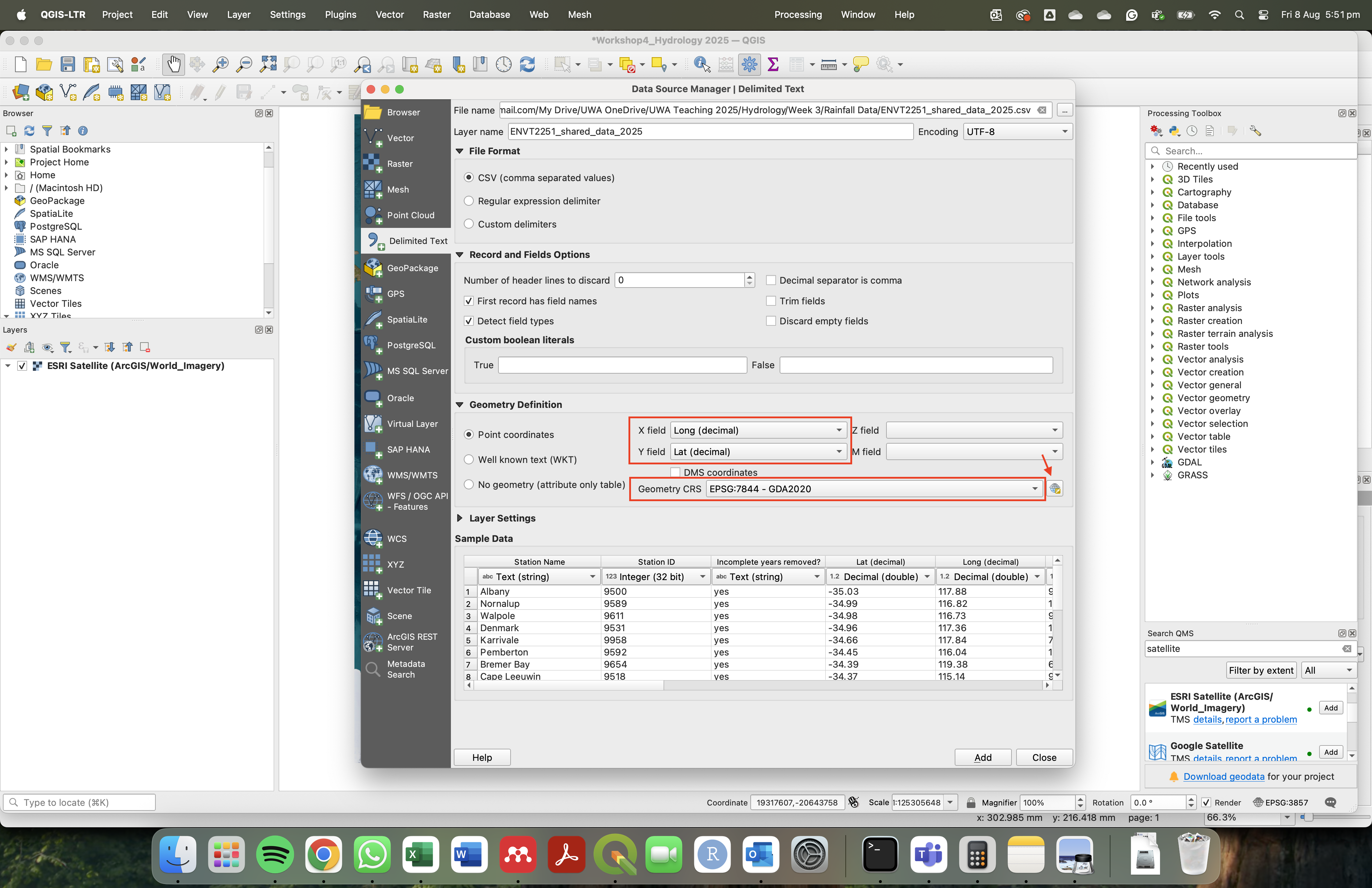
Figure 10: Settings to import data to the map.
- Once the layer is added check the points are in the right place Right click -> Zoom to layer
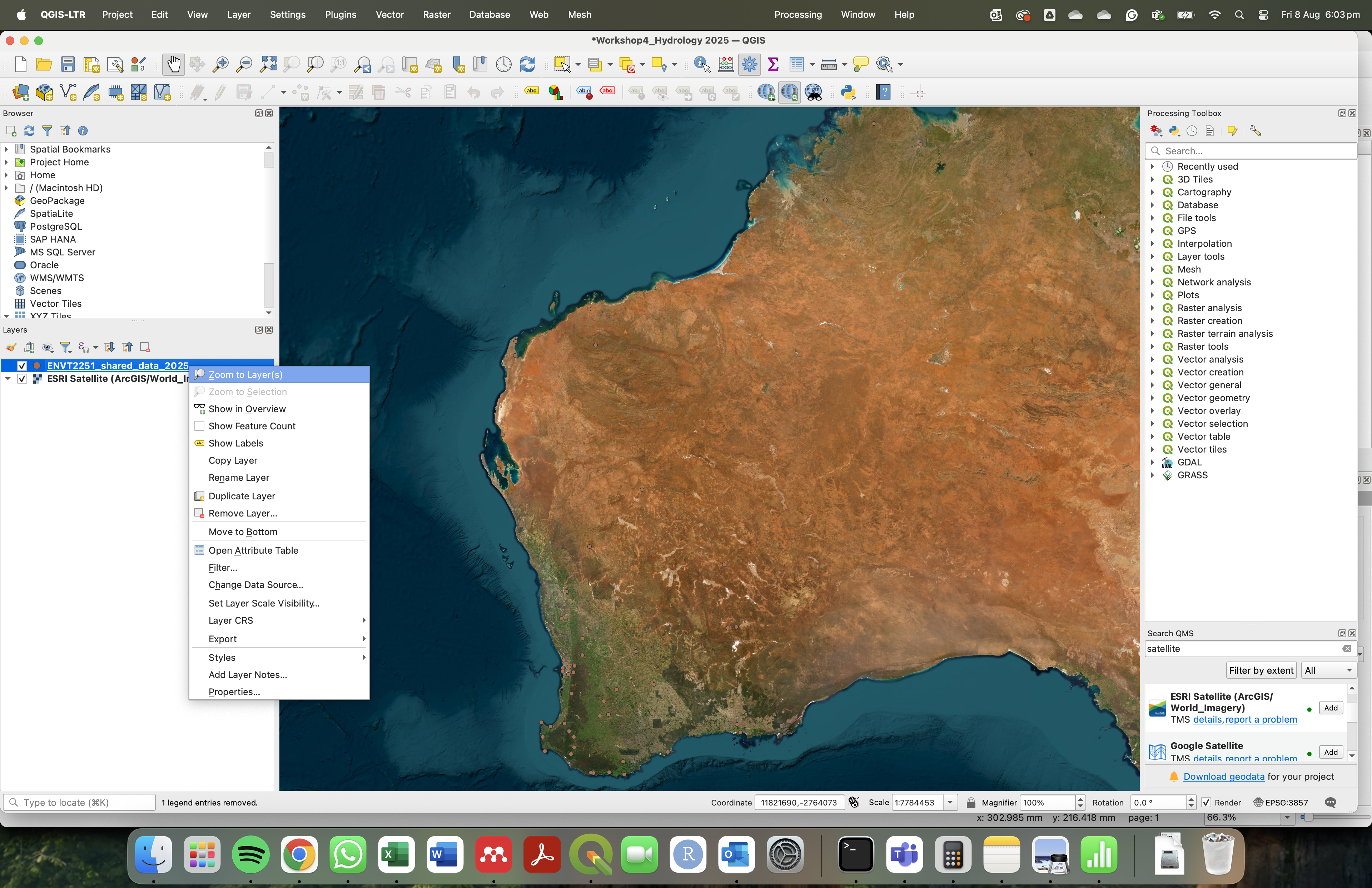
Figure 11: Zoom to layer on your map.
Now we have a basemap and our points - let’s change the symbology of the points to better communicate the variation in EC.
- Right click on the point data in the layer window and go Properties -> Symbology.
- Set the symbol type to Graduated and specifying the values to graduate by as our rainfall property column of interest.
- Now set the Method to Size, and the Mode to Natural Breaks (Jenks), click Classify.
- To change colours Right click Symbol -> Change colour.

Figure 12: Setting symbology of the layer.
Now when you click Apply the point size is weighted to the property you are showing. You can further refine your symbology by changing the point colours and size - think about how best to communicate variation in your items.
- Finally, create a map output by clicking the New Layout button in the toolbar. If you aren’t familiar with creating maps in QGIS work with one of your classmates who is, or read through the second half of this tutorial.
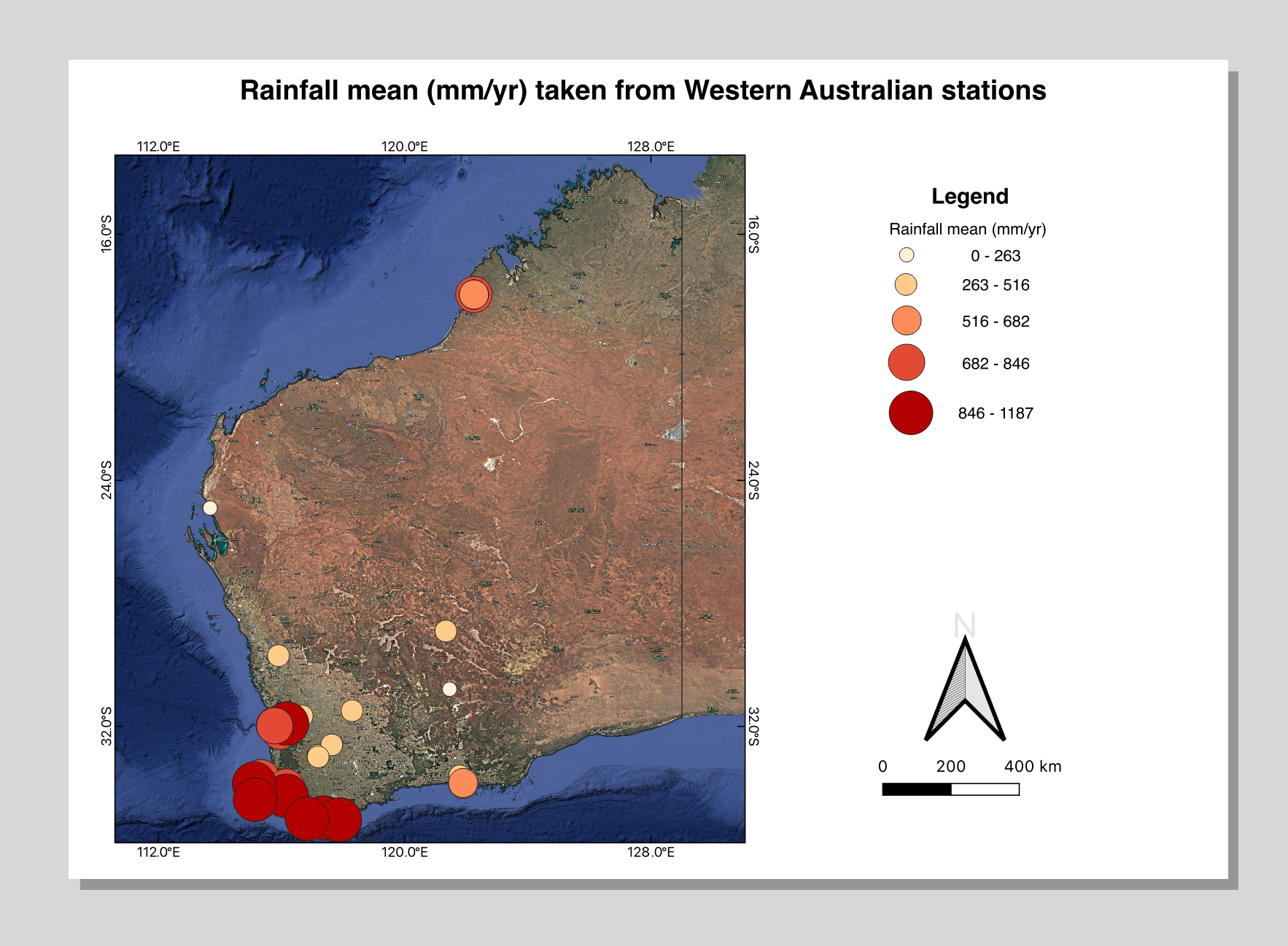
Figure 13: Example map from your QGIS output.
17) OK - you beauty! Now you have some nice visualisations of the spatial patterns (rather than the temporal ones), for different metrics of interest to our analysis. What spatial patterns do you notice? Do they match what you would expect? What may be causing these spatial patterns?
Contexualising your work
Until now, we have undertaken our own analysis of available rain and streamflow data. When writing up our work it is important for us to also contexualise our analysis relative to the prior work of others (i.e. how do our conclusions compare to what has previously been reported).
18) Spend some time to identify prior papers and reports that explain the climatology of Western Australia and any that have reported on rainfall changes and/or changes in streamflow. Try comparing search results from different portals such as traditional searches in UWA’s OneSearch, Google Scholar, and even AI-assisted searches through Chat-GPT. Do you notice the main references being consistent across the search methods? Try different search prompts to see how this can help improve the results that are returned. Remember - you are smarter than the computer!
19) These searches may yield a lot of entries so now you must critically consider which ones are most relevant to include. Could you identify some that are more relevant than others? Consider things like spatial relevance (region versus state versus continental scale?), and things like how well cited the report is (number of citations) and also the age of the article. Once you have identified a strong list, consider how you can use these within your discussion, to place your work in context of prior findings.
Assignment 1A submission
Your submission for this assessment is a summary report outlining the results of the analysis and questions posed in steps 1-19, spanning across Exercises 2,3 and 4. This should include figures and tables you have created, summarising the data from your chosen site, and also using the broader class data-set where appropriate.
Your report should have a title and the information should be grouped into numbered headings and sub-headings, like a scientific journal article.
It will start with an introduction, and have 4 data sections: 1) temporal trends in rainfall, 2) spatial patterns in rainfall, 3) interannual variability in rainfall and 4) relationship between rainfall and runoff. Finally, you should write a conclusion that summarizes the main findings and links back to the objectives you stated in your introduction.
A draft template to get you started is provided in the download link.
Make sure that all the text in your figures is legible and up to scientific standard. For charts, all axes should be clearly labeled and units given where appropriate. Make sure to include appropriate captions to describe your tables and figures, and cite these in the text (Figure captions go below the figure. Table captions go above the table).
You will be assessed according to the rubric provided on LMS. Be sure to submit your report via the Turnitin Link on LMS by the due date and time. Late submissions will attract penalties in line with UWA policy.