Appendix D : Sediment Data | The Coorong Dynamics Model

Sample points

A rich dataset with many types of data were collected along the length of the lagoon, shown in 9.67. These sites are referred to throughout this document and catalogued here on one section to create an overview. The grab samples (24) and rapid assessments (50) were taken at many points and provided one snapshot in time, in the surface sediment only. The grab samples were taken at the same points as almost half of the rapid samples and were submitted for many assays, such as total metals, as well as sediment quality. The rapid assessment samples were assessed for texture, colour and oxic/sulfidic state. Seven extra particle size samples were taken, which complement the sediment texture data from the grab samples. Five sites had cores taken in two seasons and used to measured sediment-water fluxes, as well as concentration-depth profiles. Macro invertebrate samples were taken at seven points, and one sample was transplanted to an eighth point. Finally, particle fluxes were measured at the site Villa de Yumpa.

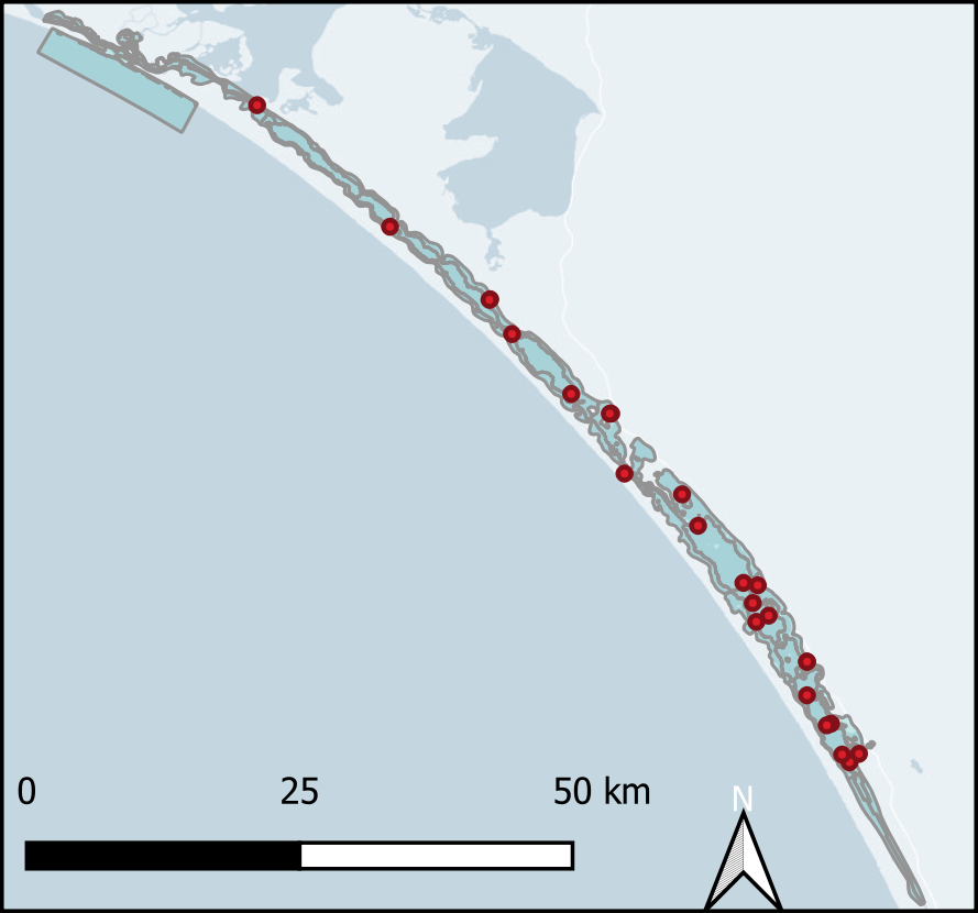
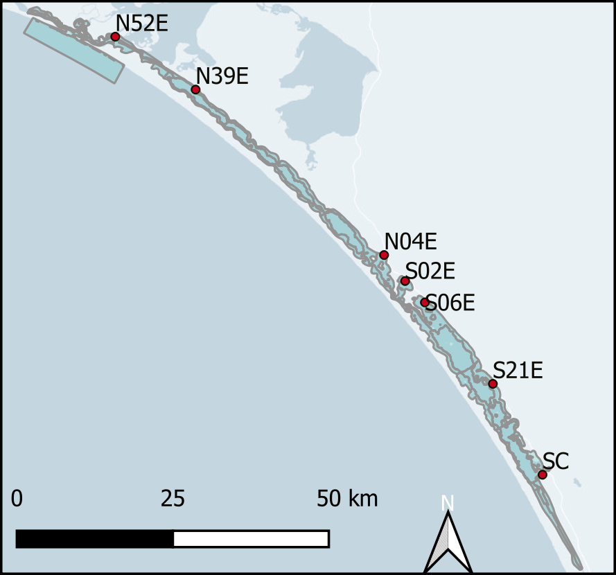
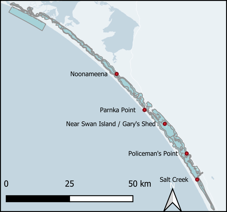
Overview of the locations and different types of sediment sample data across the Cooorong. Left - Grab samples. Centre - Particle size samples. Right - Cores.

Figure 9.67: Overview of the locations and different types of sediment sample data across the Cooorong. Left - Grab samples. Centre - Particle size samples. Right - Cores.

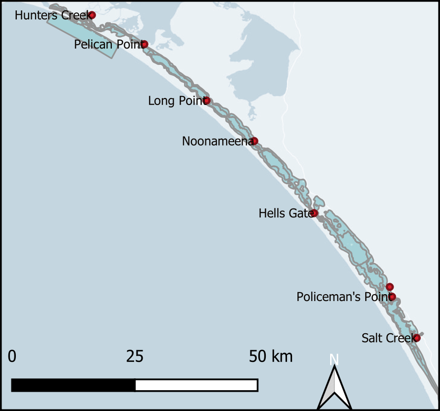
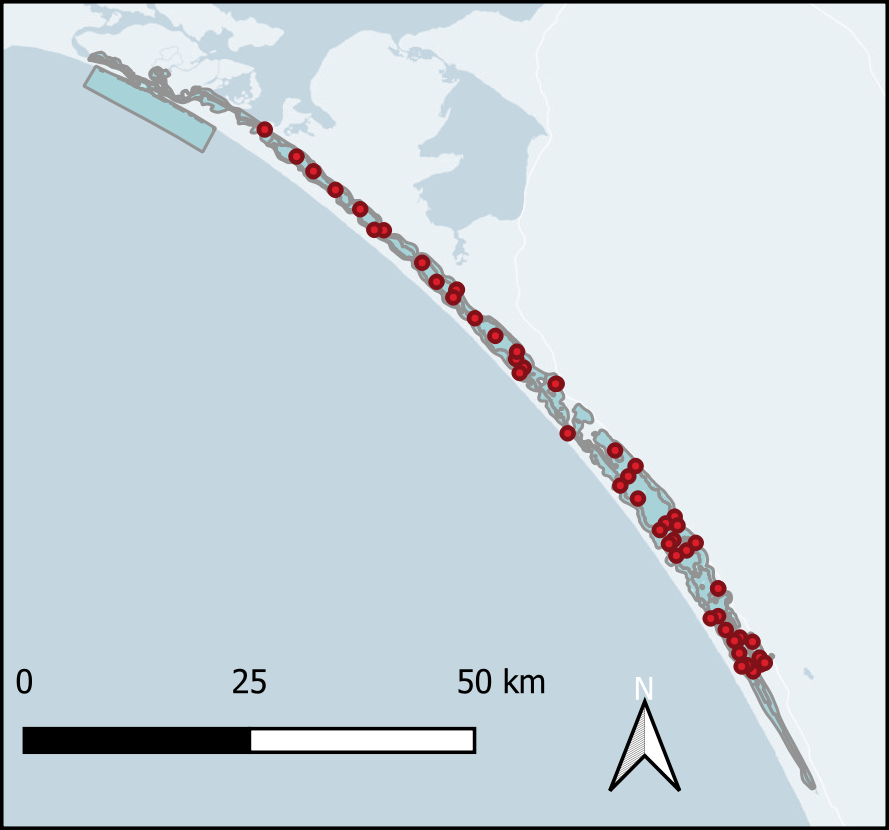
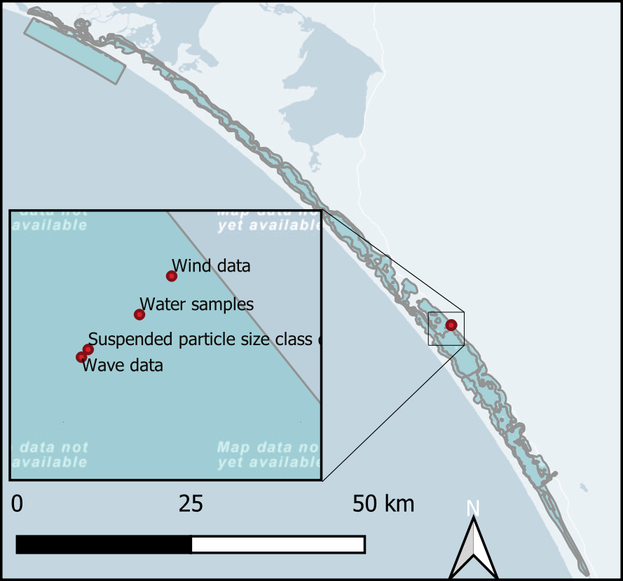
Overview of the locations and different types of sediment sample data across the Cooorong. Left - Macroinvertebrates. Centre - Rapid assessments. Right - Flux chamber.

Figure 9.68: Overview of the locations and different types of sediment sample data across the Cooorong. Left - Macroinvertebrates. Centre - Rapid assessments. Right - Flux chamber.

Sediment quality

Two sediment quality surveys by the University of Adelaide provided sediment quality data along the length of the lagoon (Figure 9.69). 24 grab samples were measured for % moisture, and proportions of gravel, sand, silt and clay. Seven other samples were taken for grain size analysis in classes of gravel, coarse sand, medium sand, fine sand, very fine sand and mud. These measured points were categorized to represent the ten Coorong zones, as well as deep and shallow areas.

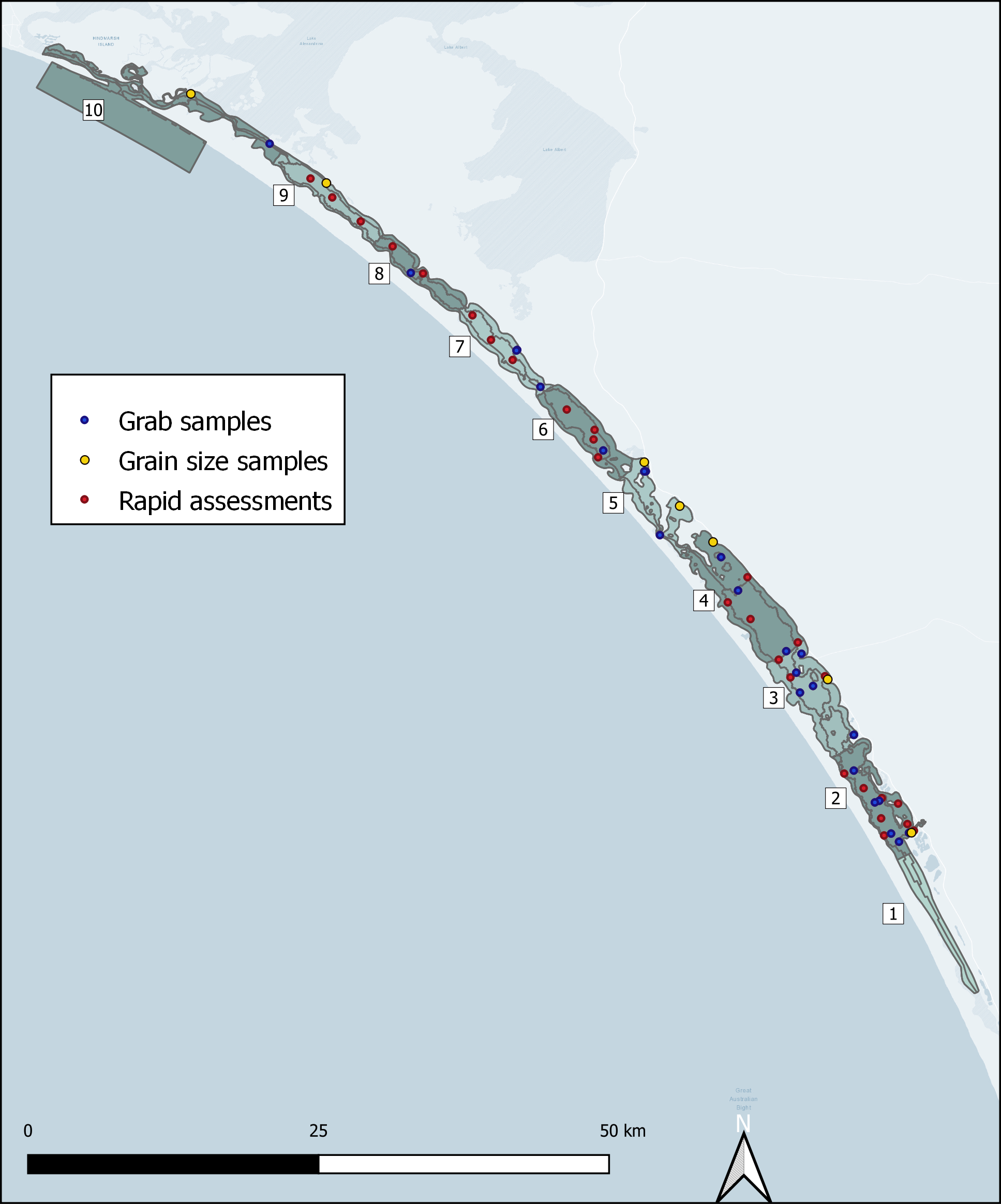
Figure 9.69: Locations of the three types of sediment quality data sampling points. In this appendix, zone numbers refer to the north-south allocation of zones before subdivision into bank/shallow zones. Hence 1 refers to 11, 12 and 13, 2 refers to 21, 22 and 23 etc.

The sediment quality points are summarised in 9.17. The sediment quality was either sand with low % moisture and low organic matter, clay with high moisture and high organic matter, or somewhere in between these (9.18). The zones that had a combination of these were further refined according to depth.

Table 9.17: Summary of sediment quality classifications for each of the 31 zones.
Zone	Sediment quality	Sand (>50 µm)	Silt (2 to 50 µm)	Clay (<2 µm)	% TOC	Water quality
104						Seawater
103	Very coarse sand Macroinvertebrates high Sandy loam	98.3	0	1.7		Freshwater
103
102		88.6	0.8	10.6	1.51	Freshwater
102	Moisture medium
101
93	Coarse sand	99.9	0	0.1		Freshwater
92	Mud (rapid = 2)
91
83
82	Macroinvertebrates high (recovered) Clay Moisture medium	49.8	0.3	49.9	2.8	Freshwater
81
73	Moisture low Sand Macroinvertebrates medium	94.5	2.5	3	0.5	Saline
72	Sandy loam	81.5	2.2000000000000002	16.3	1.5	Saline
72	Moisture medium					Saline
71
63
62	Clay Moisture high	5.4	11.5	83.1	6	Saline
61
53	Fine sand, sandy loam	90	1	9	2.2999999999999998	Hypersaline
52	Macroinvertebrates medium					Hypersaline
52	Mud (rapid = 0)					Hypersaline
51	Sandy clay Moisture medium	53.5	7.2	39.4	4.8	Hypersaline
43	Fine sand	99.8	0	0.2		Hypersaline
42	Clay Moisture high	2	10	88	7	Hypersaline
41	Mud (rapid 0)					Hypersaline
33	Sand Moisture low	93	1	6	2.2000000000000002	Hypersaline
32	Clay	27	7	67	6.8	Hypersaline
32	Moisture high					Hypersaline
31	Sandy clay Moisture medium	60.1	5.4	34.6	8.1999999999999993	Hypersaline
23	Moisture low Macroinvertebrates low	93	1	6	7.3	Hypersaline
23	NA					Hypersaline
22	Clay Sand	14	18	69	9.6	Hypersaline
21	NA					Hypersaline
21	Moisture low Sand	94.8	0.1	5	7.4	Hypersaline
13
12
11

Table 9.18: Most common combinations of texture, moisture and organic matter across the samples.
Texture	%Moisture	%Organic matter
Sand	Low	Low
Clay	High	High (~3%)
Mix	Medium	Medium (~1%)

The % moisture data was calculated as the mass of water per total mass of sample. This measurement ranged from around 20% for sandy sediment to around 80% for clay sediment. Assuming a dry mass density of 2.7 kg L^-1, these values translated to roughly 40% porosity for sand and 92% porosity for clay. The rapid assessments had a texture description converted to a scale of 1 to 5, where 1 represented sticky ooze and 5 represented coarse grains 9.70). The dominant texture type was assigned by zone. This was further refined for the bank and channel subzones.

Table 9.19: Rapid assessment criteria, based on Hallett et al. (2019). These samples assessed the grainy or oozy state of the sediment.
Criteria	5	4	3	2	1
Colour	Yellow/brown to depth of core	Yellow/brown overlying grey	Yellow/brown overlying black	Grey to depth of core	Black to depth of core
Texture	Coarse grainy	Fine grainy	NA	Smooth and silky	Oozy and slick/sticky
Odour	No odour of H₂S	Mild odour of H₂S	NA	Moderate odour of H₂S	Strong odour of H₂S

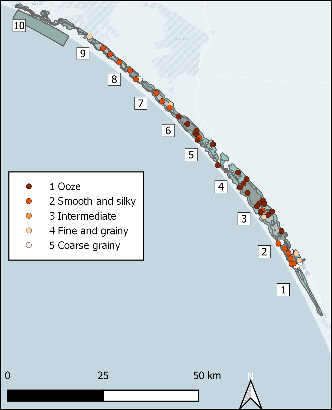
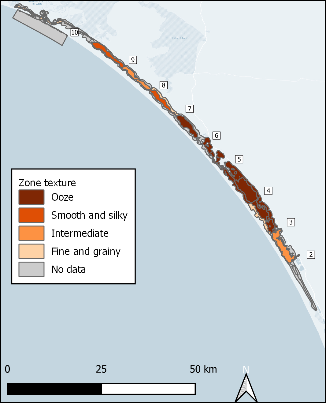
Figure 9.70: Left - sediment texture measurements from the rapid samples. Right - Texture classifications assigned to zones.

Salinity

The salinity in the southern lagoon was much higher than in the northern lagoon, due to the evaporation of the water between rainfall events (9.71). The Goyder Institute T&T report suggested that high salinity had destroyed habitat for macroinvertebrates (see also section Macroinvertebrates). Salinity was measured in the grab samples 0 to 5 cm deep. It is displayed in (9.71) as interpolated sediment salinity. Note that it is hypersaline even in the northern lagoon, in zone 6.

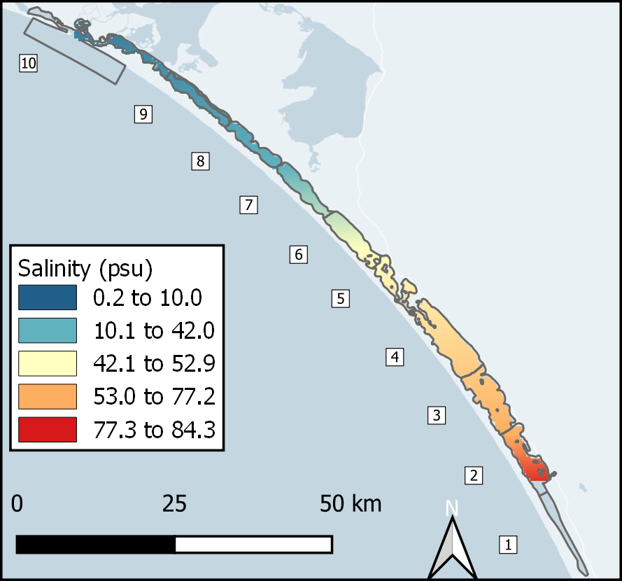
Figure 9.71: Interpolated salinity in the bottom water, performed by the University of Adelaide. Salinity is higher in the southern lagoon. For comparison, seawater is about 35 psu. The colour band only applies to the lagoon in the map, not the lakes, the ocean or zone 1.

Sulfur

The rapid assessments gave the general oxic/sulfidic state of the sediment, where the ooze texture usually coincided with the sulfidic state of the sediment (see criteria in 9.20. These were divided per zone (9.72) and further divided by depth. There were no measurements of $SO_4^{2-}$ in the sediments or the water column, and so an estimate was made by correlating the $SO_4^{2-}$ concentration with salinity.

Table 9.20: Rapid assessment criteria, based on Hallett et al. (2019). These samples indicate the sulfidic state of the sediment.
Criteria	5	4	3	2	1
Colour	Yellow/brown to depth of core	Yellow/brown overlying grey	Yellow/brown overlying black	Grey to depth of core	Black to depth of core
Texture	Coarse grainy	Fine grainy	NA	Smooth and silky	Oozy and slick/sticky
Odour	No odour of H₂S	Mild odour of H₂S	NA	Moderate odour of H₂S	Strong odour of H₂S

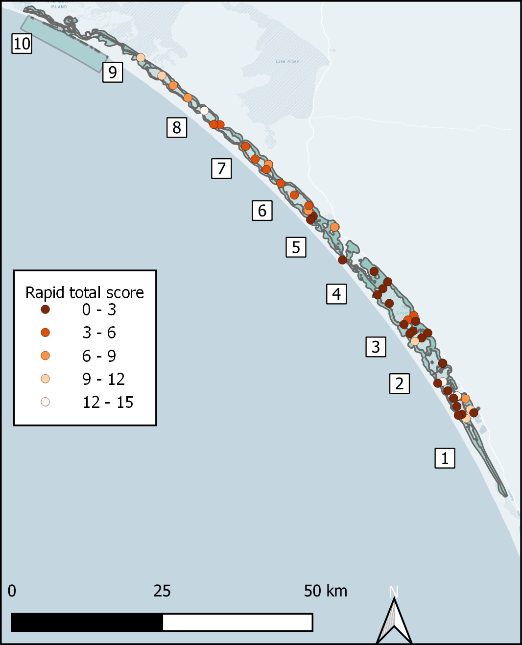
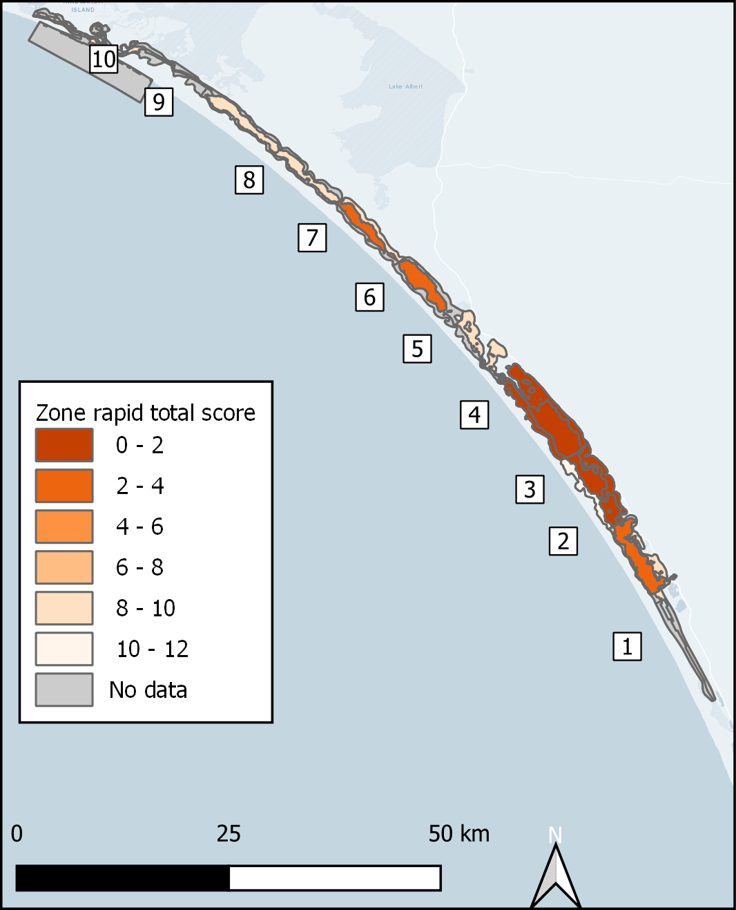
Rapid tests in the Coorong, which indicate sulfidic state of the sediment. Left – Individual rapid assessment points; Right – rapid scores averaged across points in zone.

Figure 9.72: Rapid tests in the Coorong, which indicate sulfidic state of the sediment. Left – Individual rapid assessment points; Right – rapid scores averaged across points in zone.

Table 9.21: H₂S core sites and times.
	November 2020	February 2021
Noonameena	Day/night
Parnka Point	Day/night	Day/night
Near Swan Island		Night
Policeman’s point	Day/night	Day/night
Salt Creek		Night

Nutrients

The grab samples also provided TN and TP measurements. These are shown as interpolated data (9.73). Nutrients were concentrated in zones 4 and 6, either side of the narrow, shallow zone 5 that separates the north and south lagoons.

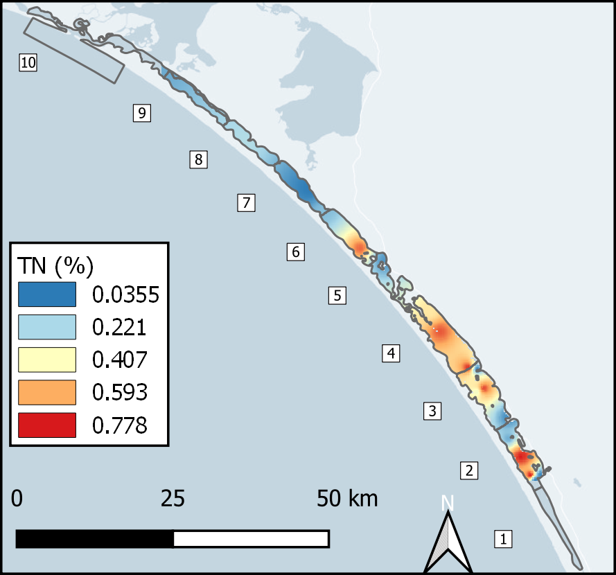
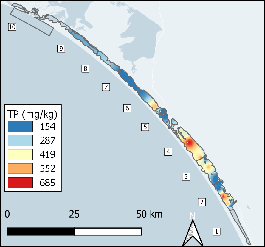
Figure 9.73: Interpolated nutrients as calculated by University of Adelaide. Left - TN (%). Right - TP (mg kg^-1),

Nutrients were measured in cores at three locations (9.74. While $NH_4^+$ was present in all cores, $PO_4^{3-}$ was below the detection limit at two of the points (in zones 2 and 7), and only above the detection limit at Parnka Point (zone 5). Note that zone 2 had high TP but low $PO_4^{3-}$, therefore it must be examined whether there were high concentrations of organic P. The $NH_4^+$ concentration reached around 0.1 mmol L-1 and the $PO_4^{3-}$ 0.01 mmol L-1 (9.75).

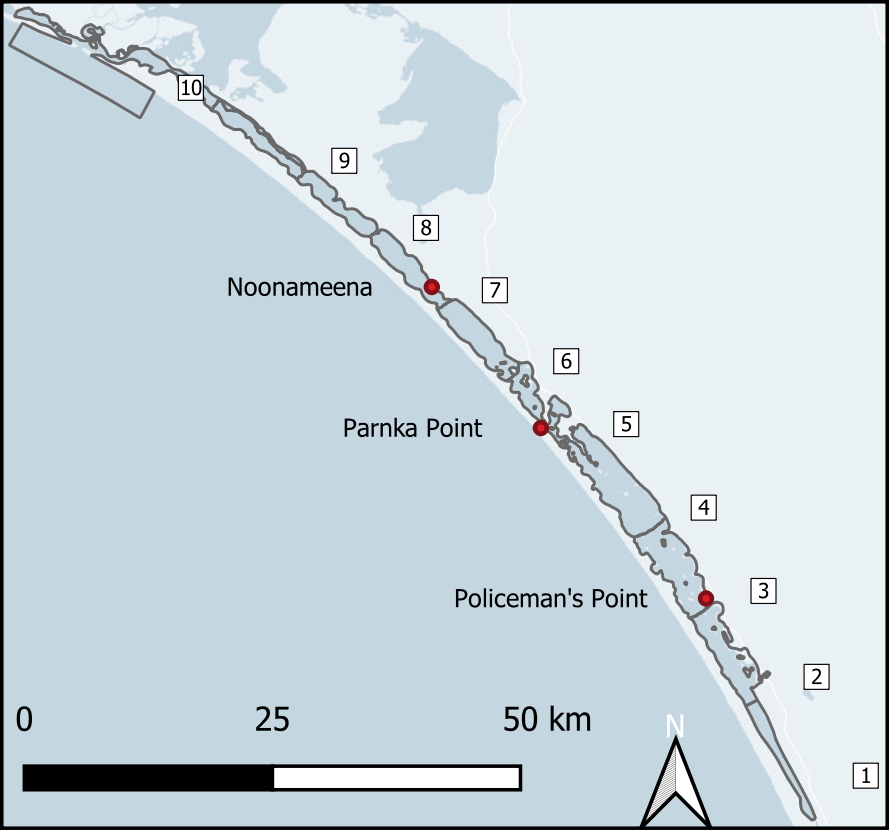
$Sampling sites for nutrient cores, in which $NH_4^+$ and $PO_4^{3-}$ profiles were measured to 12 cm depth.$

Figure 9.74: Sampling sites for nutrient cores, in which $NH_4^+$ and $PO_4^{3-}$ profiles were measured to 12 cm depth.

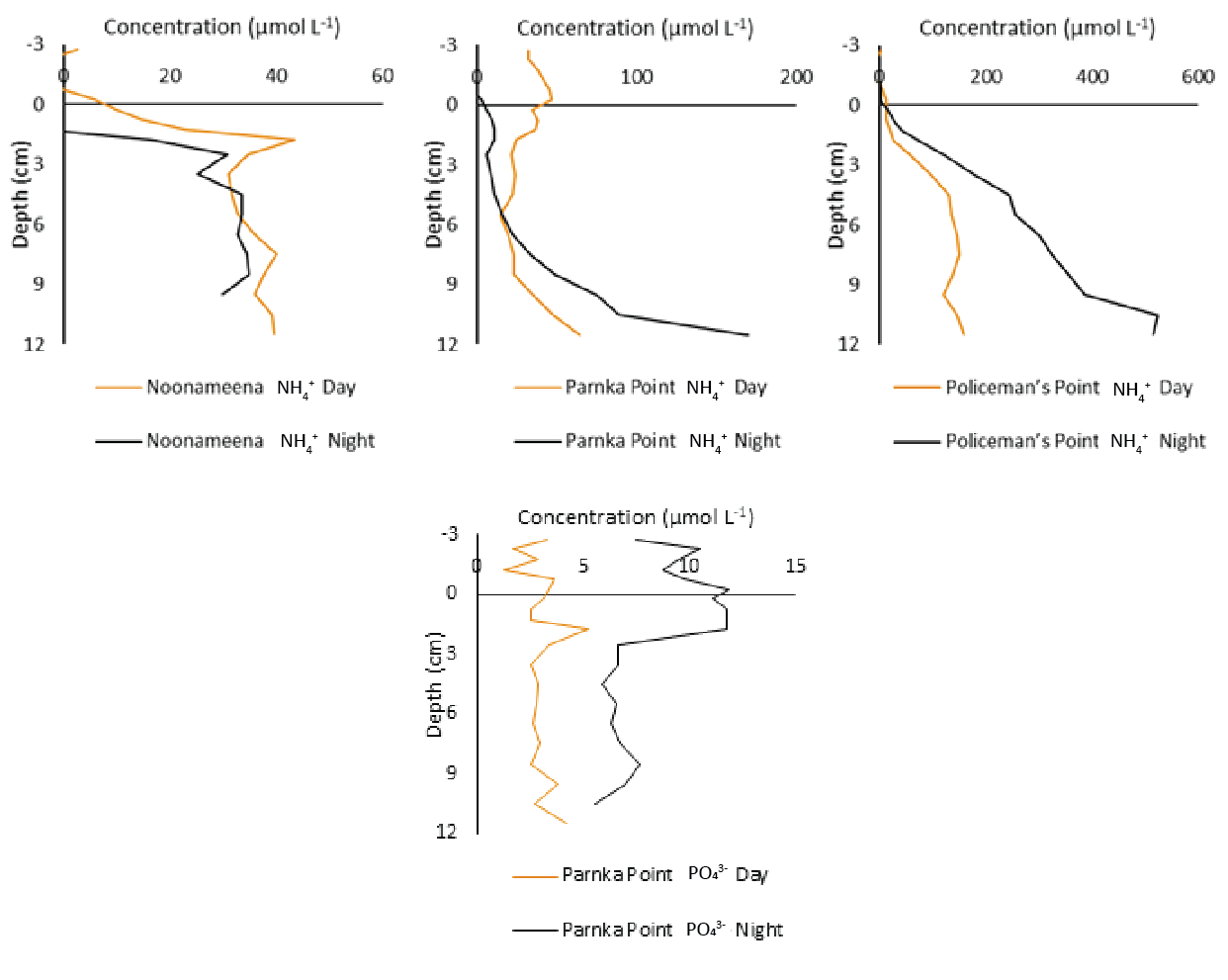
$Measured $NH_4^+$ and $PO_4^{3-}$ cores. $PO_4^{3-}$ was below detection limits for Noonameena and Policeman's Point sites.$

Figure 9.75: Measured $NH_4^+$ and $PO_4^{3-}$ cores. $PO_4^{3-}$ was below detection limits for Noonameena and Policeman’s Point sites.

Table 9.22: Measured nutrient fluxes from Parnka point (mmol m^-2 y^-1). The negative NH₄⁺ dark value indicates that it fluxes from the water column to the sediment.
Time	NH₄⁺	NO₃^-	PO₄^3-
Dark	-9298	25	229
Light	2221	2340	0

Oxygen

The rapid assessment sites give an indication of whether the sediment was oxic (high value) or sulfidic (low value) (9.76). Zones 3, 4, 6 and 7 were the least oxic.

Rapid tests in the Coorong, which indicate oxic state of the sediment. Left – Individual rapid assessment points; Right – rapid scores averaged across points in zone.

Figure 9.76: Rapid tests in the Coorong, which indicate oxic state of the sediment. Left – Individual rapid assessment points; Right – rapid scores averaged across points in zone.

Oxygen fluxes were measured at two sites, Parnka Point and Policeman’s Point (9.77). At each site, there were five cores. Each core was incubated for one to three hours in either light or dark conditions. The oxygen concentration in the headspace was measured. Parnka Point cores had concentration around 6 mg L^-1, or 180 µmol L^-1. This site had sandy sediment with low concentrations of organic matter and nutrients. (This was the same point that produced nutrient cores and fluxes.)

Policemans Point cores had concentration of 5 mg L^-1, or 150 µmol L^-1. This site had either clay or sand, with high concentrations of organic matter, nutrients, and sulfidic ooze. In all dark cores, the concentration dropped slightly. In all Policeman’s Point light cores concentration increased. In the Parnka Point light cores, results were mixed: in three cores the concentration decreased and in two cores the concentration increased. There are four oxygen fluxes to work within (9.23). Note that Parnka Point has a narrower range of flux and is still negative in the light conditions. Policeman’s Point has a wider range and positive oxygen flux under light conditions.

Table 9.23: Oxygen flux (mol m^-2 y^-1). Negative values indicate that the oxygen fluxes from the water column to the sediment. The positive value indicates that the sediment produced oxygen and fluxes it to the water column
Time	Parnka Point	Policeman’s Point
Dark	-9298	-19693
Light	-3150	3552

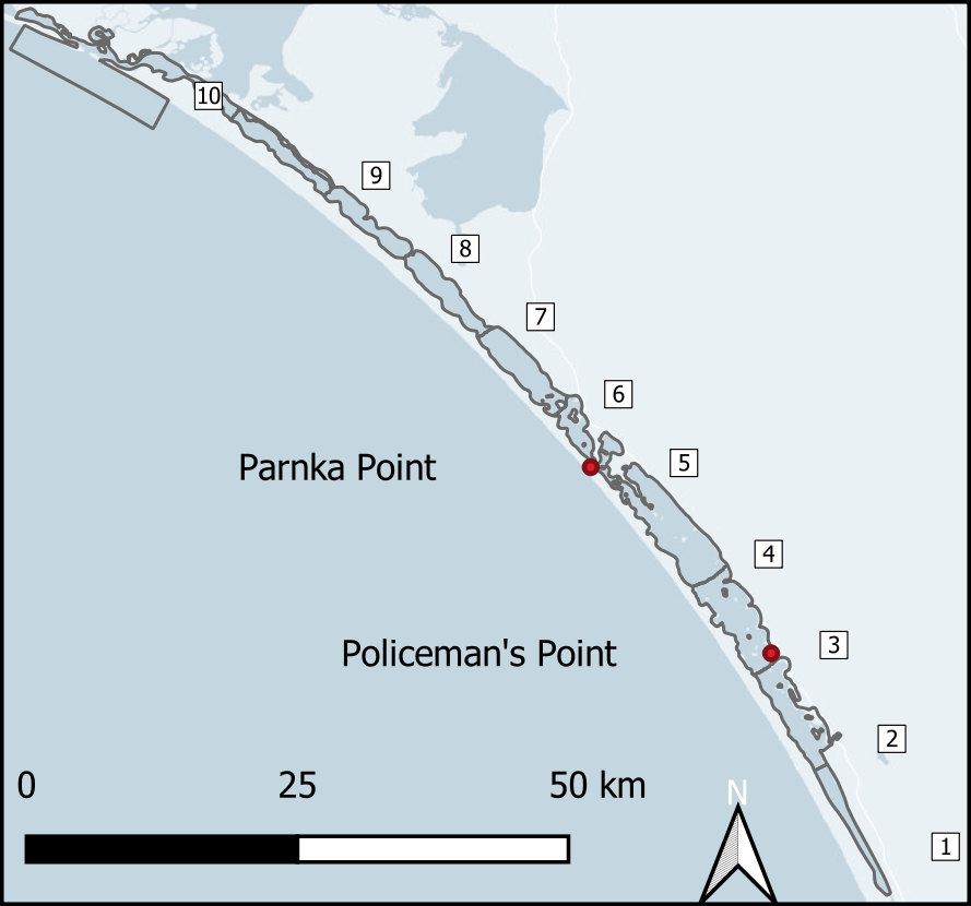
Figure 9.77: Locations where $O_2$ fluxes were measured.

Organic matter

The grab samples provided a measure of total organic carbon (TOC). The highest areas mapped onto the areas of high nutrients (9.78).

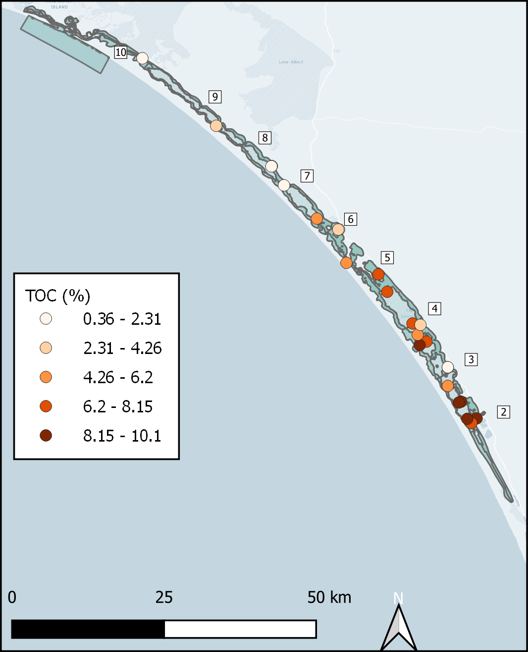
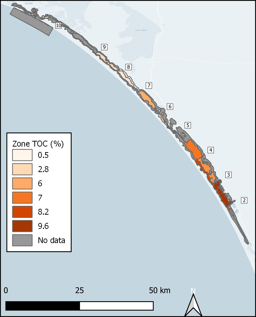
Figure 9.78: TOC% from the grab samples. Left - Individual grab samples for TOC%. Right - TOC % applied to zones.

TOC % was converted to organic matter (mmol L^-1) according to the following rationale: - TOC % was measured as kg OC per kg dry sample (and the raw value was divided by 100).
- The kg dry sample was converted to L of total sample as (%moisture / 100 + 2.7 × (1 - %moisture / 100)), where %moisture was measured at each site and 2.7 was the value assumed for kg solids per L solids.
- The kg OC was converted to mol OC by dividing by 12 g / mol and multiplying by 1000 for g OC.
- The mol OC / L was multiplied by 1000 for mmol OC / L total.
- The mmol OC / L total was divided by 0.35 to get the total organic matter concentration.
- The value 0.35 was derived by assuming a molecular formula of (CH₂O)_A(NH₃)_B(H₃PO₄)_C where the ratio A:B:C was assumed to be 106:16:1. Although there were total C and N measurements in the sediment data, there were no measurements of organic C:N:P ratios and so the assumed value was used.

Macroinvertebrates

Macroinvertebrate populations were measured at seven locations (9.79). The northernmost two sites (zones 10 and 9) had high abundance. Noonameena (zone 7) had moderately low abundance. The southernmost sites (zones 5 and 2) had very low abundance. The variable that explained this pattern was the hypersalinity (T&I reference document). A sample was taken from Jack Point (zone 2) and transplanted to Long Point (zone 8).

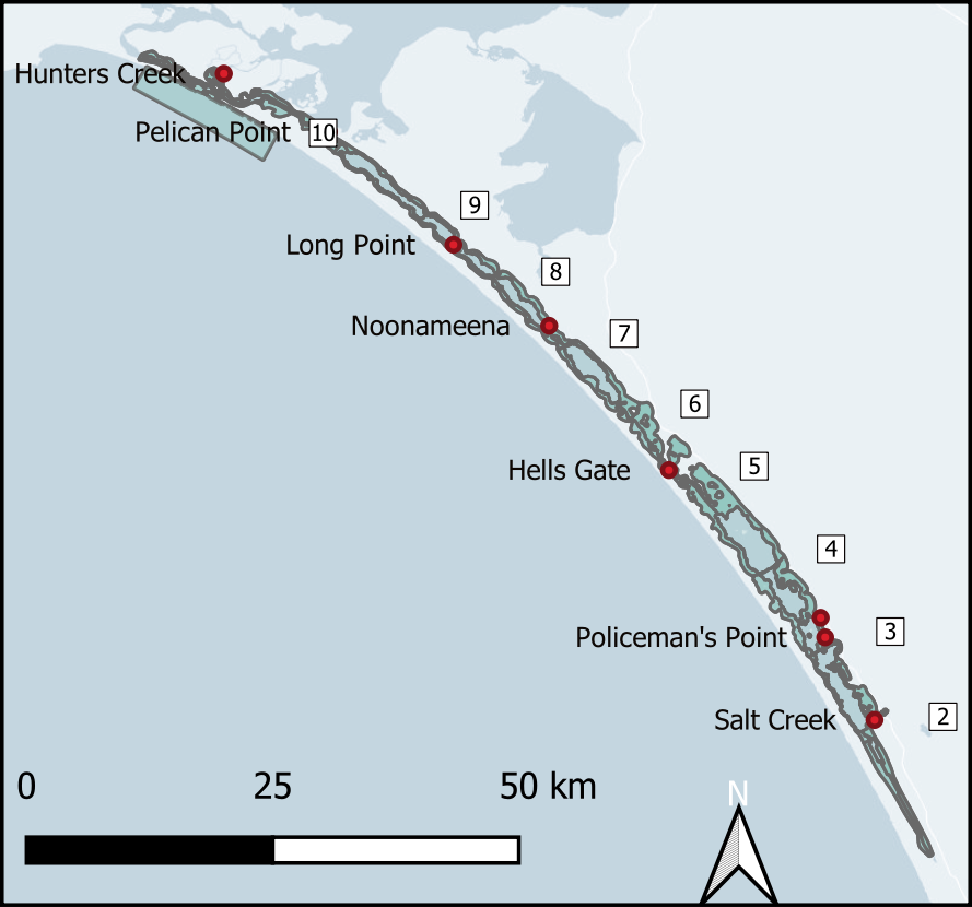
Figure 9.79: Sampling sites for macroinvertebrate measurements.

Iron and manganese

Total iron and manganese data were available from the grab samples (9.80).

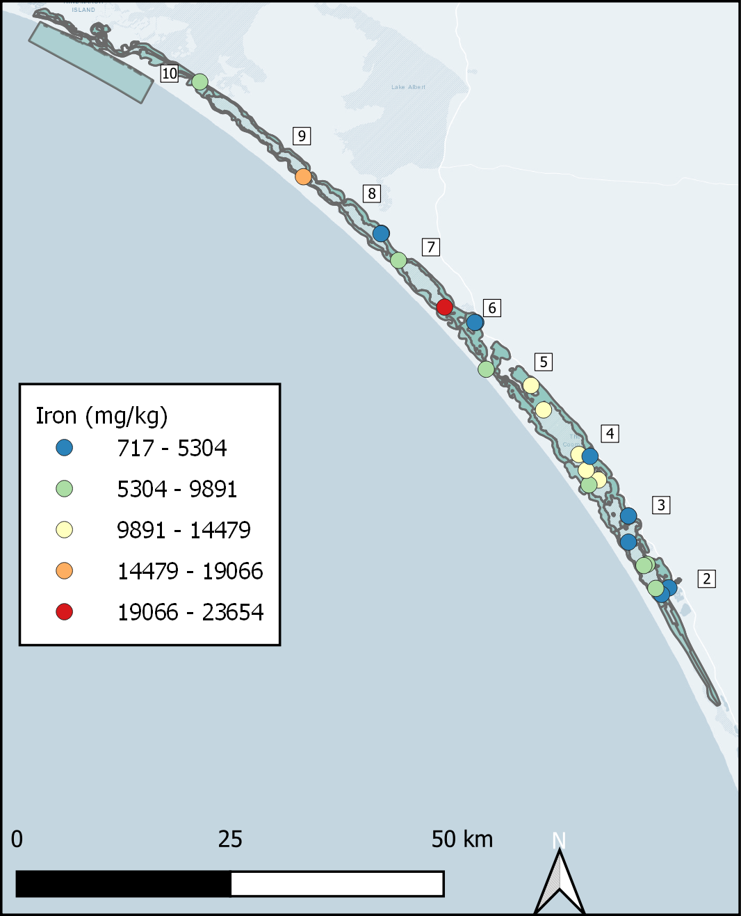
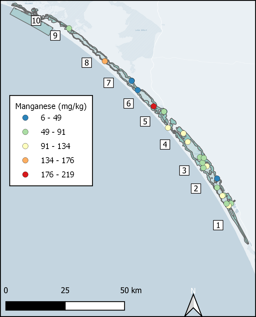
Figure 9.80: Left - Total iron from grab samples. Right - total manganese from grab samples.

Cores were taken from five locations, in November 2020 and February 2021 (9.81) and $Fe^{2+}$ was measured (Table 10). The presence of $Fe^{2+}$ indicates iron reduction of organic matter. The highest concentrations were at Parnka Point (zone 5) and Policeman’s Point (zone 3) in November 2020. These were not sites that had very high TOC or nutrients.

Table 9.24: Times and locations of cores where $Fe^{2+}$ samples were taken.
	November 2020	February 2021
Noonameena	Day/night	Night
Parnka Point	Day/night	Day/night
Near Swan Island		Night
Policeman’s point
South of Salt Creek

Table 9.25: Approximate concentrations of $Fe^{2+}$ in core samples.
	November 2020	February 2021
Noonameena	0.01	0.020
Parnka Point	0.1	0.010
Near Swan Island		0.005
Policeman’s point	0.15	0.020
South of Salt Creek		0.030

$Sampling locations for cores where $Fe^{2+}$ profiles were measured.$

Figure 9.81: Sampling locations for cores where $Fe^{2+}$ profiles were measured.

$Concentration profiles of $Fe^{2+}$.$

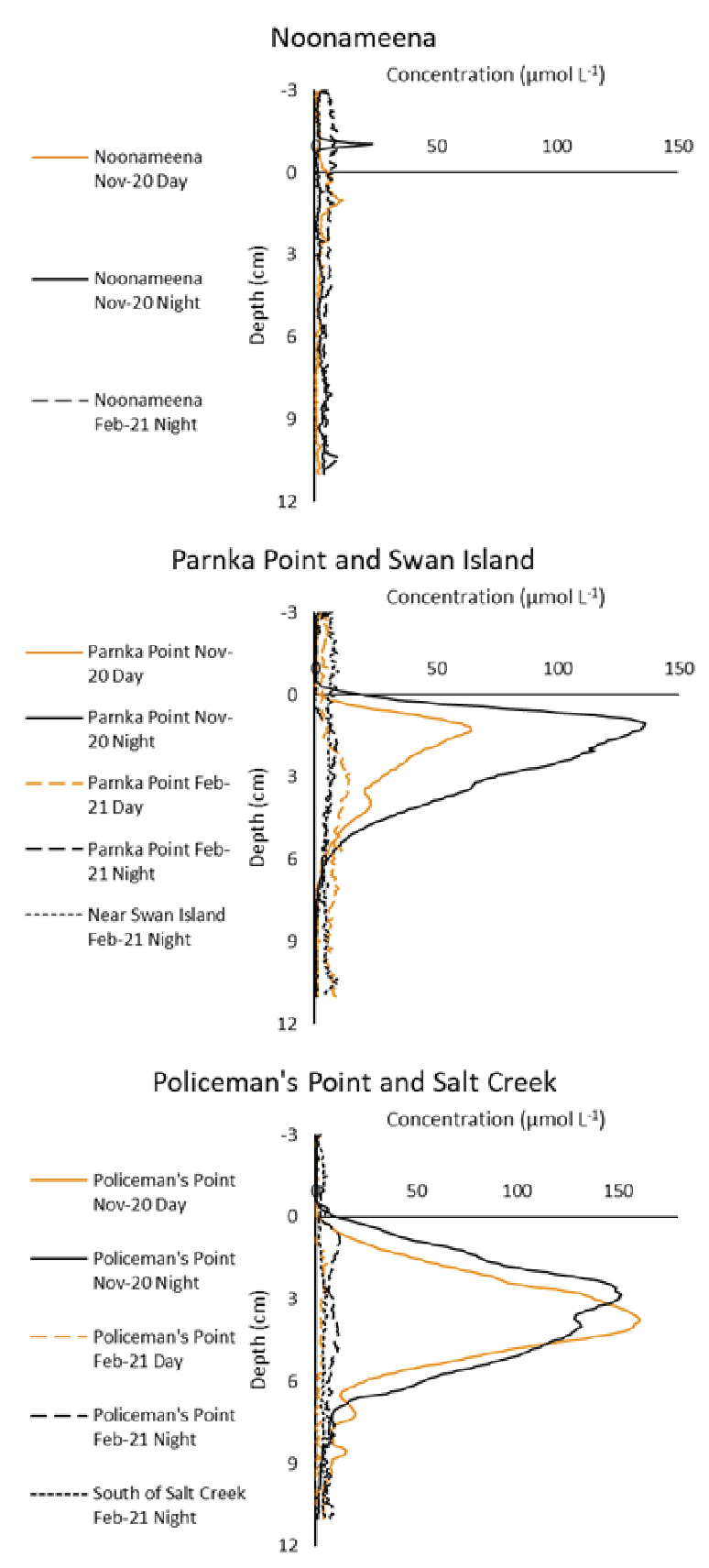
Figure 9.82: Concentration profiles of $Fe^{2+}$.

Iron data was also available from the water column sampling to use as a boundary at the sediment water interface. As with $SO_4^{2-}$, since the water column model did not simulate iron and so an approximation was taken from measured data. Data was available for total iron and dissolved iron (mg L^-1), at 16 sites along the whole Coorong, for the time period 1998 to 2012. The dissolved iron was typically less than 1% of the total iron. Both were converted to mmol L^-1 and averaged over the entire time period at each site. The total iron was assumed to be particulate iron and it was converted from mmol L^-1 to a flux in mmol m^-2 y^-1 by multiplying the concentration by the deposition rate in cm y^-1. The deposition rate was assumed to be 1 cm y-1.

Iron sulfides

FeS and FeS₂ are likely to be present in the sediments of the Coorong, however, they were not measured directly. Measurements of acid volatile sulphide (AVS) were taken with each grab sample by the field researchers. It was decided to attempt to connect AVS with FeS concentration, while still weighing the uncertainty of the connection.

An argument has been presented by Rickard and Morse (2005) that measured AVS is not necessarily a good proxy for FeS, because of differences in what is being measured at study sites. The AVS may not correspond to all of the sulphide in the sediment, it may correspond to different metal sulphide species and it may be partly organic sulphur compounds. The rapid assessments in the Coorong showed that there was a sulphurous black ooze in many of the sediment samples and so the presence of an organic sulphur compound mixed with metal sulphur compounds is possible. Several responses to Rickard and Morse’s paper were published in the same issue, including one from Meysman and Middelburg, which presented the issue from the point of view of sediment diagenesis modellers. Meysman and Middelburg’s perspective on modelling reflected the model used for this project well. They wrote that although Rickard and Morse’s explanation is thorough and precise, it is not necessarily helpful for modellers, who cannot include all chemical species in their models, especially if there is not measured data for calibration. Considering this argument, the authors of this paper pursued the AVS measurement.

AVS was converted from units of ‘% S WW,’ which was assumed to be kg S (100 kg wet sediment)^-1, to mmol S (L total volume)^-1, using porosity at each grab site. (A sample of 0.025 % S WW converted to 3.7 mmol S L^-1, where the porosity was 0.66). The average of the AVS grabs was 3.36 mmol L^-1, the minimum value 0.26 and maximum 7.21 mmol L^-1.

The AVS concentrations in the grab samples mostly corresponded with the values in the rapid assessments, with high concentrations usually in the deep channel and in zones 4, 5 and 6.

The AVS concentrations were compared to the total iron concentrations from the grab samples. The average total iron was 7.69 mmol L^-1 total sediment, which implies roughly two Fe for each S on average over the lagoon. Each site did not have a clear correlation between S and Fe. Therefore it would be hard to justify an assignment of FeS concentration based on AVS. A compromise approximation was reached in which the FeS concentration was assigned as total Fe minus AVS. The remaining Fe was assigned as Fe(OH)₃.

pH and alkalinity

pH was generally high, with an average of 8.72, across the grab samples. This was likely a result of the high amounts of shell grit in the surface sediment, corresponding with the high scores in the rapid assessments. Inorganic carbon was measured as the difference between %Total carbon minus %Total organic carbon. The maximum value was in zone 2 at the inland edge, and the minimum value was in zone 6 in the channel.