6 Macroalgae
6.1 Overview
Recent surveys in the Coorong have highlighted the challenge to ecosystem health due to the high biomass and wide extent of filamentous algae, and these ‘blooms’ have become emblematic of the recent cycle of eutrophication experienced in the lagoon (Figure 6.1). The survey data highlight that the filamentous algae, mainly species from the genus Ulva, are tightly associated with the locations where the seagrass Ruppia is present, and they flourish in areas with shallow, warm and poorly-mixed water. Late in the season the smothering and deoxygenation caused by the breakdown of large Ulva biomass accumulations drives poor water quality. This section describes the approach to simulating macroalgae within the CDM, and development of the model to tailor to the observed data collected within the HCHB research program.
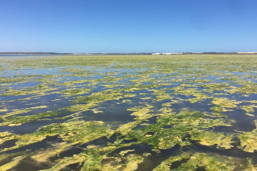
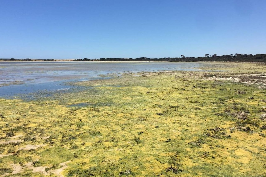
Figure 6.1: Images of filamentous algae bloom conditions within the Coorong South Lagoon, showing the pervasive extent of biomass accumulation. Photo credit: David Paton.
6.2 Model approach
Within the Coorong, the AED model has previously been set up to predict inorganic and organic nutrients, and chlorophyll-a. Whilst nutrients are not directly required for the Ruppia model assessment, the presence of filamentous algal blooms can compete for light and these are linked to bioavailable nutrients within the water column (in addition to other attributes).
6.2.1 Filamentous algae
We include a filamentous algae variable, \(FA\), in the model that is customized to reflect the Ulva community that was been extensively described. For this case we assumed it to be attached to benthic substrate, and is therefore is not subject to advection and mixing, but can slough off under high stress conditions and become a floating variable subject to transport. Evidence from the field suggest the abundance of filaments are tightly linked to the Ruppia shoots, which the algae use to anchor too.
In general, the balance equation describes how the biomass changes over time, according to:
\[ \frac{d\left(FA\right)}{dt}=+f_{\text{uptake}}^{FA}-f_{\text{excr}}^{FA}-f_{\text{mort}}^{FA}-f_{\text{resp}}^{FA}\ -f_{\text{slough}}^{FA} \tag{6.1} \] where the main growth term is resolved as:
\[ \scriptsize{f^{FA}_{\text{uptake}} = \underbrace{R^{FA}_{\text{growth}}}_{\text{max growth} \\ \text{rate at 20$^\circ$C}} \ \ \underbrace{(1-k^{FA}_{\text{pr}})}_{\text{photorespiratory} \\ \text{loss}} \ \ \underbrace{\Phi^{FA}_{\text{tem}}(T)}_{\text{temperature} \\ \text{scaling}} \text{min} \left \{\underbrace{\Phi^{FA}_{\text{light}}(I)}_{\text{light limitation}}, \underbrace{\Phi^{FA}_{\text{N}}(NO_{3},NH_{4})}_{\text{N limitation}}, \underbrace{\Phi^{FA}_{\text{P}}(PO_{4})}_{\text{P limitation}} \right \} [FA]} \tag{6.2} \]
An example of the above approach in practice is shown in the below animation. The results highlight, for this time period of interest, the areas where salinity exceeds the threshold and initially limits the productivity, and the shallow areas where light is abundant; along with other environmental drivers (e.g., temperature) these shape the biomass accumulation pattern seen in the top left panel. Animations like this for different periods throughout the year, or between years, can look quite different.
6.2.2 Macroalgae growth physiology
The original AED macroalgal biomass model previously applied in the Generation 0 and 1 CDM applications, and exemplified in the above example, has been further developed to include advances to light extinction within the canopy, nutrient cycling and excretion processes, and updates to the parameterisations associated with photosynthesis and biomass accumulation. The latter, in particular, are updated to better align with the experimental work reported in Waycott et al. (2019) and recent survey data collected as part of from the HCHB research program.
The algal biomass, \(FA\) (or \(MAG_C\)), is simulated in units of carbon (\(mmol\:C/m^2\)), and in addition the groups have been configured to have a variable C:N:P ratio. The model therefore tracks the internal cell nutrition and includes dynamic uptake rates of N and P sources simulated in response to changing water column conditions and internal nutrient stress.
The growth rate functions used in Eq (6.2) are tailored to use temperature and salinity ranges based on the experimental data reported in Waycott et al. (2019).
6.2.3 Resolving seasonal life-stage dynamics
Following review of the initial data and findings from the T&I project 2, the approach to modelling macroalgae has been revised to better resolve seasonal shifts in form and physiology over the seasonal cycle.
A new ‘colony’ based model for simulating clump emergence, biomass accumulation and sloughing has been conceptualised (Figure 6.2). The model adopts the same underlying physiology as described in the above section, but allows for age/size specific application of these rates to better align with recent observations and monitoring.
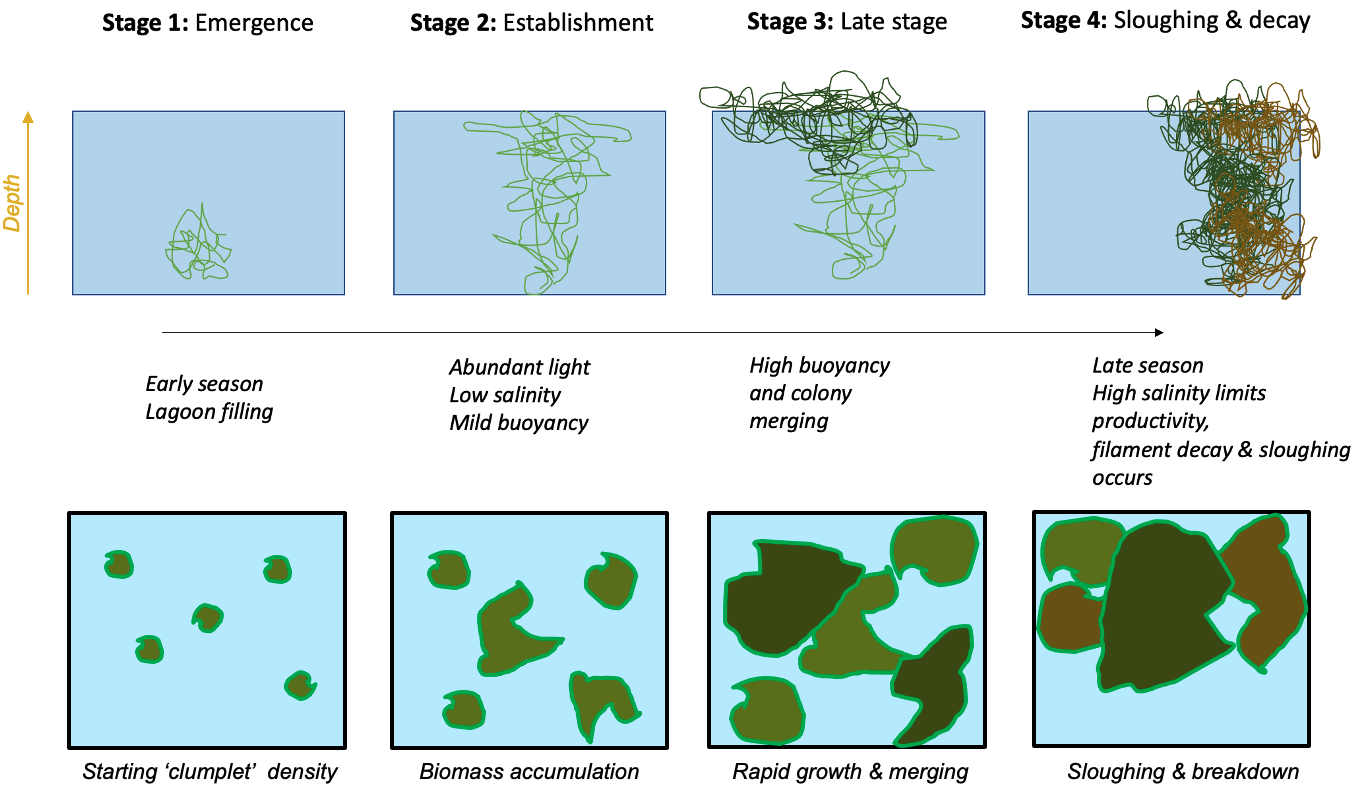
Figure 6.2: Schematic depicting a new life-stage based macroalgal “clump” model developed to track seasonal macroalgal biomass development stages and late-stage decay.
This approach allows more direct links with a) the experimental data collected on biomass accumulation and photosynthesis rates in the lab, and b) the field data estimates of macroalgae density from photos and aerial imagery at different points through the growth season.
The approach essentially follows a size-class based model for resolving the filamentous algae biomass pool. According to the above conceptual schematic, four discrete life-stage (aka size) categories are included. In general they are fixed in space, but note that ‘sloughed’ biomass (Stage 4) becomes mobilised after a sloughing ‘event,’ and can continue to be exposed to surface light irradiances and also begin decomposition should environmental conditions be inadequate for growth (e.g., as the water becomes too salty).
The fundamental balance equation shaping growth remains as depicted in Eq (6.1) to capture the various processes impacting ulva growth and decay, with the difference that each growth-stage allows for different light, nutrient and salinity sensitivity, and there is a aging component linking the size classes, \(R_{aging}\). A full description of the AED macroalgae model can be referred to the AED science manual.
6.2.4 Ulva HSI
In addition to the simulation of Ulva biomass, a simple “Habitat Suitability Index” (HSI), termed \(Ulva\:HSI\), was also developed to map Ulva growth potential and ‘hotspot’ locations. The \(Ulva\:HSI\) is an index between 0 and 1, and is computed by normalising the expression outlined in Eq (6.2). This metric does not account for the accumulation of biomass, or consider processes such as mortality and sloughing or mobilisation, but is a useful metric to look where high growth rates typically occur.
6.3 Data availability
6.3.1 Algae extent within the lagoon
Regular monitoring for macroalgae biomass within the Coorong is not routinely undertaken, but a range of data are available over the model calibration and testing periods. A summary of the available algal extent data is summarised in Table 6.1.
| Identifier | Description | Date range | # sites |
|---|---|---|---|
| Historical monitoring | |||
| UA MDBA_1 |
Algae presence/absence; Water depth (categorical) |
2017 May | 8 |
| UA ORH |
Algae No/Rare/Present/Extreme; Water depth; Salinity |
2016 Dec | 24 |
| HCHB surveys | |||
| UA HCHB seasonal |
Estimated algae biomass (7 categories); Algae cover% (0/20/40/50/60/80/100); Water depth; Salinity |
2020 Sep - 2021 Dec | ~100 each season |
The locations of the various smaplign campaigns for assessment of Filamentous Algae presence and biomass are shown for the historical (pre-HCHB) sampling campaigns (Figure 6.4) and for the more intensive sampling campaigns undertaken within the HCHB research program (Figure 6.3).
HCHB Monitoring A summary of the HCHB Filamentous Algae monitoring locations are shown below.
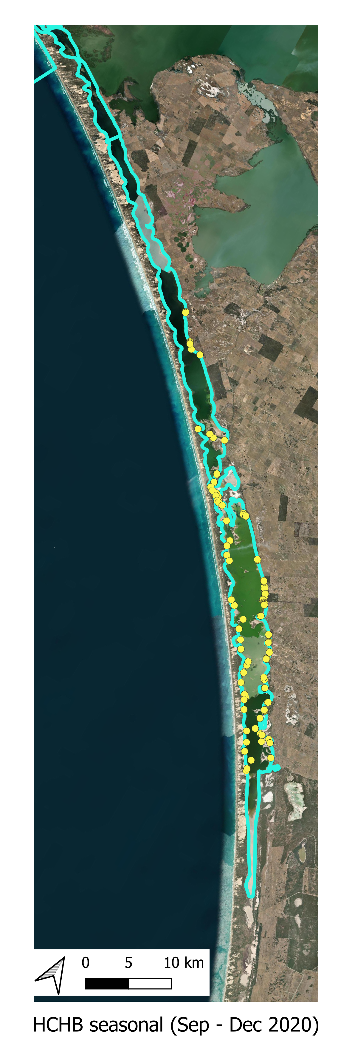
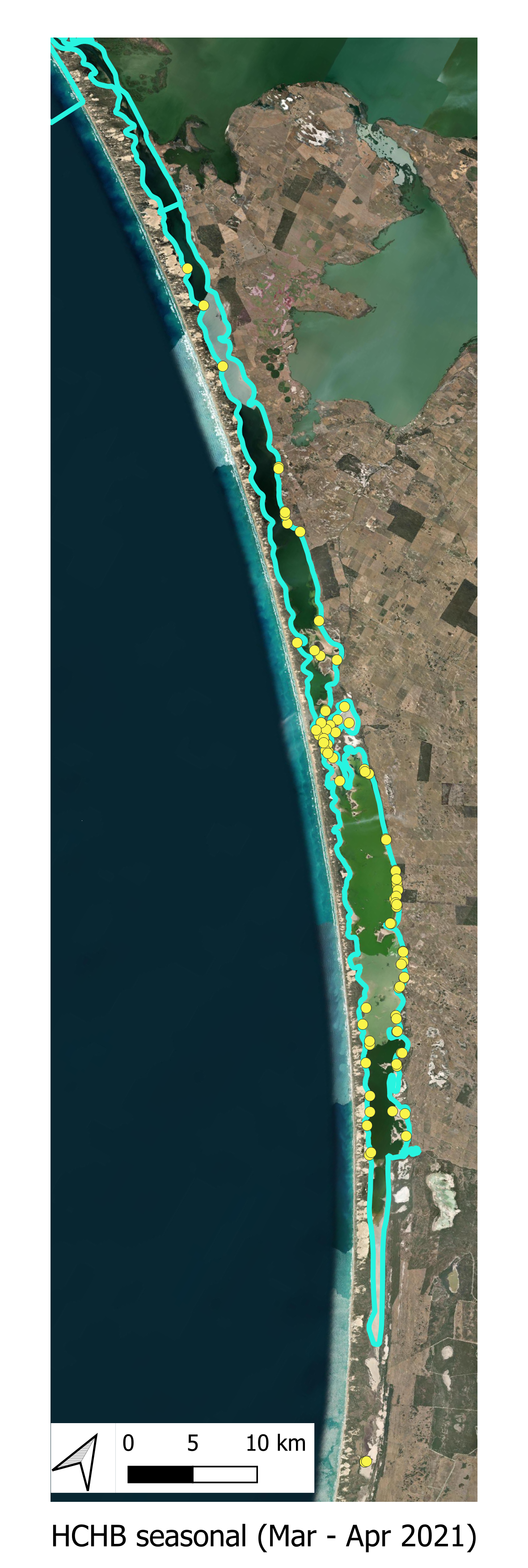
Figure 6.3: Filamentous algae sampling sites for the HCHB program (T & I 2). Agency/program code under each map corresponds to those listed in Table 6.1. Turquoise outline represents the model boundary. Click image to enlarge.
Historical Monitoring A summary of historical (pre 2020) Filamentous Algae monitoring locations are shown below.
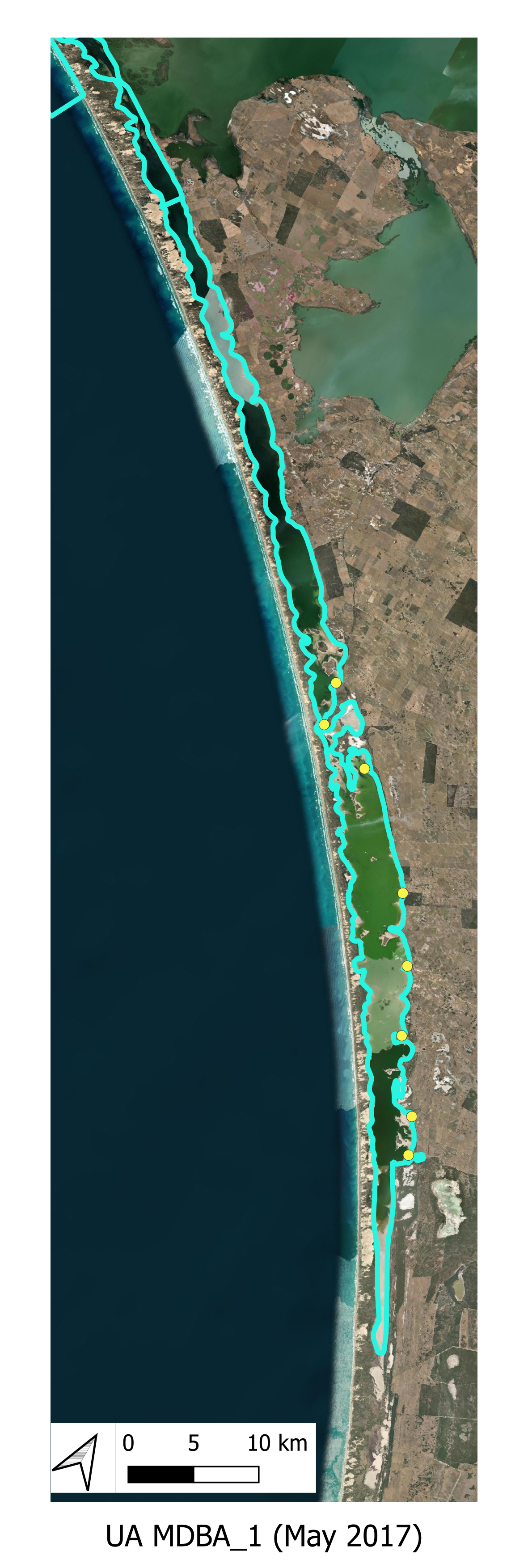
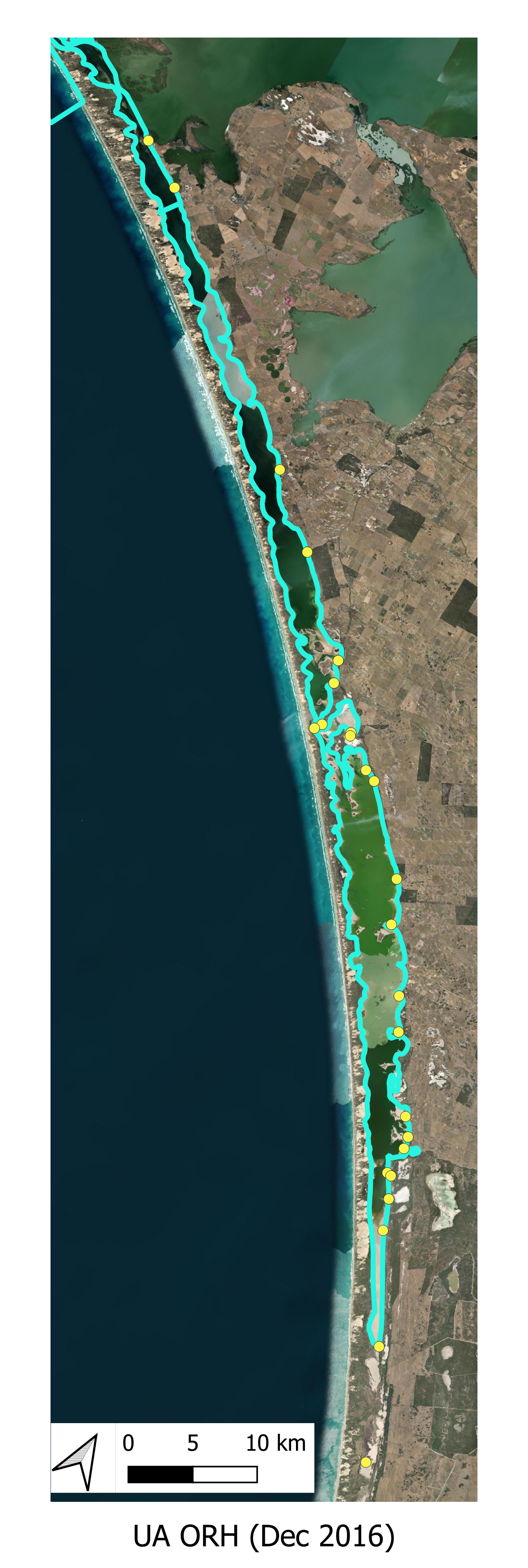
Figure 6.4: Filamentous Algae sampling sites for monitoring program prior to 2020. Agency/program code under each map corresponds to those listed in Table 6.1. Turquoise outline represents the model boundary. Click image to enlarge.
6.3.2 Environmental threshold parameter review
In order to set/refine the parameters required for the macroalgae model, such as light, salinity and temperature responses, a review of available experimental data and observations was undertaken. The key information sourced incldued:
- For salinities from 35—90 ppt, an optimum temperature for the Ulva paradoxa filamentous green algal community was 30°C, which was the temperature where the relationship between weight gain became the most positive (Waycott et al., 2019).
- At salinities of 30 - 140 ppt, weight change decreased as salinity increases. Salinities of more than 90 ppt were the most significant at reducing filamentous green algal growth rates. At a salinity of 140 ppt the growth of algae is inhibited at all temperatures (Waycott et al., 2019).
- At salinities below 35 g/L, algal communities appear resilient to a wide range of temperatures and nutrient availability Asanopoulos and Waycott (2020).
6.4 Model setup
Four pools were configured to simulate the biomass of filamentous algae, \(ulva_a\), \(ulva_b\), \(ulva_c\) and \(ulva_s\). The parameters used in the setup are outlined in Table (Table 6.2).
| Parameter | Description | Unit | Parameter1 | Parameter2 | Parameter3 | Parameter4 |
|---|---|---|---|---|---|---|
| General | ||||||
| \[m\] | name of macroalgal group | \[\small{-}\] | ‘ulva_a’ | ‘ulva_b’ | ‘ulva_c’ | ‘slough’ |
| \[MAG |_{t=0}\] | initial concentration of macroalgae | \[\small{mmol\: C/m^2}\] | 10 | 10 | 10 | 10 |
| \[MAG_0\] | minimum concentration of macroalgae | \[\small{mmol\: C/m^2}\] | 0.2 | 0.2 | 0.2 | 0.2 |
| \[\chi_{C:chla}^{MAG}\] | carbon to chlorophyll ratio | \[\small{mg\: C/mg\: chla}\] | 50 | 50 | 50 | 50 |
| Growth | ||||||
| \[R_{growth}^{MAG}\] | macroalgae group maximum growth rate at \(20^{\circ}C\) | \[\small{/d}\] | 2.4 | 1.8 | 3.1 | 2.1 |
| \[\Theta_{tem}^{mag}\] | specifies temperature limitation function of growth | \[\small{-}\] | 1 | 1 | 1 | 1 |
| \[\theta_{growth}^{mag}\] | Arrenhius temperature scaling for growth function | \[\small{-}\] | 1.08 | 1.08 | 1.08 | 1.08 |
| \[T_{std}\] | standard temperature | \[\small{^{\circ}C}\] | 18 | 20 | 18 | 18 |
| \[T_{opt}\] | optimum temperature | \[\small{^{\circ}C}\] | 23 | 26 | 28 | 25 |
| \[T_{max}\] | maximum temperature | \[\small{^{\circ}C}\] | 35 | 38 | 39 | 32 |
| Light | ||||||
| \[\Theta_{lgt}^{mag}\] | switch to assign the type of light response function | \[\small{-}\] | 0 | 0 | 0 | 0 |
| \[I_K\] | half saturation constant for light limitation of growth | \[\small{W/m^2}\] | 100 | 100 | 100 | 100 |
| \[K_{e}^{MAG}\] | specific attenuation coefficient | \[\small{/m/(mmol\:C/m^2)}\] | 0.00408 | 0.0051 | 0.00408 | 0.0048 |
| \[f_{pr}\] | fraction of primary production lost to exudation | \[\small{-}\] | 0.025 | 0.025 | 0.025 | 0.025 |
| Respiration | ||||||
| \[R_{resp}^{MAG}\] | phytoplankton respiration/metabolic loss rate at \(20^{\circ}C\) | \[\small{/d}\] | 0.04 | 0.08 | 0.02 | 0.095 |
| \[\theta_{resp}^{mag}\] | Arrhenius temperature scaling factor for respiration | \[\small{-}\] | 1.08 | 1.08 | 1.08 | 1.08 |
| \[k_{fres}\] | fraction of metabolic loss that is true respiration | \[\small{-}\] | 0.1 | 0.1 | 0.1 | 0.1 |
| \[k_{fdom}\] | fraction of metabolic loss that is released as DOM | \[\small{-}\] | 0.3 | 0.3 | 0.3 | 0.3 |
| \[\Theta_{sal}^{mag}\] | type of salinity limitation function | \[\small{-}\] | -1 | -1 | -2 | -3 |
| Salinity | ||||||
| \[S_{bep}\] | salinity limitation value at maximum salinity (\(S_{maxsp}\)) | \[\small{-}\] | 0.1 | 0.1 | 0.1 | 0.1 |
| \[S_{maxsp}\] | maximum salinity where growth is possible | \[\small{g/kg}\] | 28 | 60 | 200 | 90 |
| \[S_{opt}\] | optimal salinity for growth | \[\small{g/kg}\] | 10 | 20 | 60 | 40 |
| Nitrogen | ||||||
| \[\Theta_{din}^{mag}\] | switch for the selected group to simulate \(DIN\) uptake | \[\small{-}\] | 1 | 1 | 1 | 1 |
| \[\Theta_{in}^{mag}\] | switch for the selected group to simulate dynamic intracellular \(N\) store | \[\small{-}\] | 0 | 0 | 0 | 0 |
| \[N_o\] | external \(DIN\) concentration below which uptake is 0 | \[\small{mmol\: N/m^3}\] | 0.02 | 0.071 | 0.02 | 0.071 |
| \[K_N\] | half-saturation concentration of nitrogen | \[\small{mmol\: N/m^3}\] | 1.786 | 2.143 | 1.786 | 2.4 |
| \[\chi_{ncon}^{mag}\] | constant internal nitrogen concentration | \[\small{mmol\: N/m^3}\] | 0.16 | 0.151 | 0.1 | 0.167 |
| \[\chi_{nmin}^{mag}\] | minimum internal nitrogen concentration | \[\small{mmol\: N/m^3}\] | 0.069 | 0.054 | 0.069 | 0.069 |
| \[\chi_{nmax}^{mag}\] | maximum internal nitrogen concentration | \[\small{mmol\: N/m^3}\] | 0.18 | 0.054 | 0.18 | 0.206 |
| \[R_{nuptake}^{mag}\] | maximum nitrogen uptake rate | \[\small{mmol\: N/m^3/d\: /(mmol\: C/m^3)}\] | 0.069 | 0.032 | 0.069 | 0.206 |
| Phosphorus | ||||||
| \[\Theta_{dip}^{phy}\] | switch for the selected group to simulate \(DIP\) uptake | \[\small{-}\] | 1 | 1 | 1 | 1 |
| \[\Theta_{ip}^{phy}\] | switch for the selected group to simulate dynamic intracellular \(P\) store | \[\small{-}\] | 0 | 0 | 0 | 0 |
| \[P_o\] | external \(DIP\) concentration below which uptake is 0 | \[\small{mmol\: P/m^3}\] | 0.0064 | 0.0064 | 0.0064 | 0.0064 |
| \[K_P\] | half-saturation concentration of phosphorus | \[\small{mmol\: P/m^3}\] | 0.2526 | 0.3226 | 0.2426 | 0.36 |
| \[\chi_{pcon}^{mag}\] | constant internal phosphorus concentration | \[\small{mmol\: P/m^3}\] | 0.002976 | 0.0028086 | 0.00186 | 0.0031062 |
| \[\chi_{pmin}^{mag}\] | minimum internal phosphorus concentration | \[\small{mmol\: P/m^3}\] | 0.0015 | 0.0015 | 0.0015 | 0.0015 |
| \[\chi_{pmax}^{mag}\] | maximum internal phosphorus concentration | \[\small{mmol\: P/m^3}\] | 0.0096 | 0.0096 | 0.0096 | 0.0096 |
| \[R_{puptake}^{mag}\] | maximum phosphorus uptake rate | \[\small{mmol\: P/m^3/d\: /(mmol\: C/m^3)}\] | 0.0031 | 0.0031 | 0.0031 | 0.0031 |
| \[\omega_{mag}\] | sedimentation rate | \[\small{m/d}\] | n/a | n/a | n/a | 0 |
| \[d_{mag}\] | macroalgae filament mean length scale | \[\small{m}\] | 0 | 0 | 0 | 0 |
| \[c_1\] | rate coefficient for density increase | \[\small{kg/m^3/s}\] | 0 | 0 | 0 | 0 |
| \[c_3\] | minimum rate of density decrease with time | \[\small{kg/m^3/s}\] | 0 | 0 | 0 | 0 |
The total biomass of \(FA\), in comparable units to the field data (\(g\text{ dry weight}/m^2\)), is termed \(TMALG\) and computed as the sum of the attached and floating components:
\[ TMALG = \left[\underbrace{\sum_i^{\text{a,b,c}} \left( ulva_{i} \right)}_{\text{attached}} + \underbrace{ulva_{s}\:\Delta z}_{\text{floating}} \right] \: \chi_{c:dw} \: \times 10^{-3} \tag{6.3} \] where \(\chi_{c:dw}\) is the dry weight per carbon ratio. \(TMALG\) is used to assess against the algal densities reported in the field, thus assuming the reported algal densities from the transects are the combined amount of attached and detached material.
6.5 Validation and assessment
6.5.1 Generation 0
Using the Generation 0 model, the following assessment against Ulva biomass prediction and data showing presence/absence was recorded (Figure 6.5). The simulated biomass reasonably correlated with the presence/absence data record in 2016 in particular, but included several false positives in 2017 in the South Lagoon. Whilst biomass data wasn’t recorded in the survey data for these time periods, the simulated biomass concentrations have retrospectively been seen to be systematically under predicting the typical biomass levels seen in the HCHB field surveys.
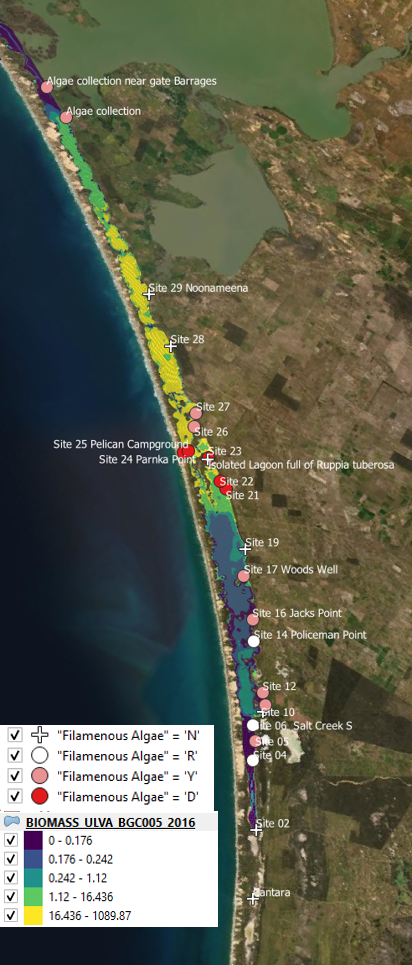
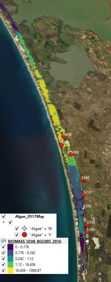
Figure 6.5: Comparison of observed and simulated Ulva for 2016 (left) and 2017 (right).
Nonetheless, the modelled \(Ulva\:HSI\) prediction correlated well with the observed filamentous algae abundance categories (Figure 6.6). This implies the growth controls (as embodied in the HSI) are well resolved, but the seasonal factors leading to biomass accumulation were more complicated, thus justifying the further refinements outlined in Section 6.3. The HSI range was however quite restricted and not as sensitive suggesting the normalisation could be improved.
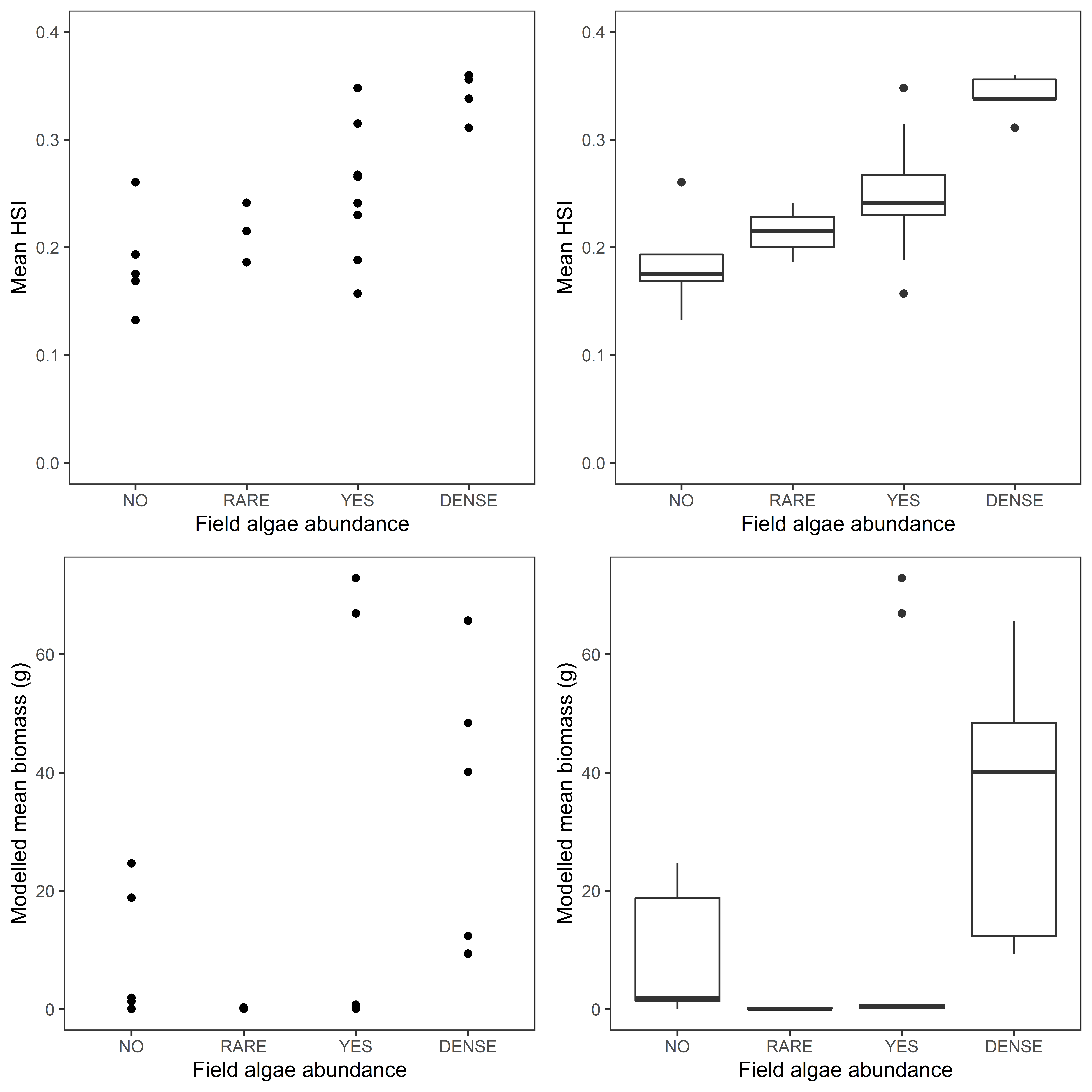
Figure 6.6: Filamentous algae observed density and equivalent model predicted Ulva HSI (top) and Ulva Biomass (bottom).
6.5.2 Generation 2.1
Following further refinement of the general water quality model calibration (as outlined in Chapters 4-5), and the macroalgae model developments (Section 6.3), the Generation 2.1 model was run over the period from 2020-2021, inclusive, and the results were compared with in-depth HCHB survey data collected during several surveys undertaken within the period (see Figure 6.3).
The model results are shown in Figure 6.7 - 6.8 for the 2020 dataset, and Figure 6.9 - 6.10 for the 2021 dataset.
The simulated biomass in this version is higher that Gen 0, around 100-200 gDW/m2 in the main zones. This is lower than some of the peak biomass densities recorded in the field. This, however, was deemed to be acceptable as the model is predicting the average biomass across broad areas in the simulated mesh, whereas the observed data shows patchy densities with areas of high and low densities, with the higher biomass recorded in the shallow areas near the shore.
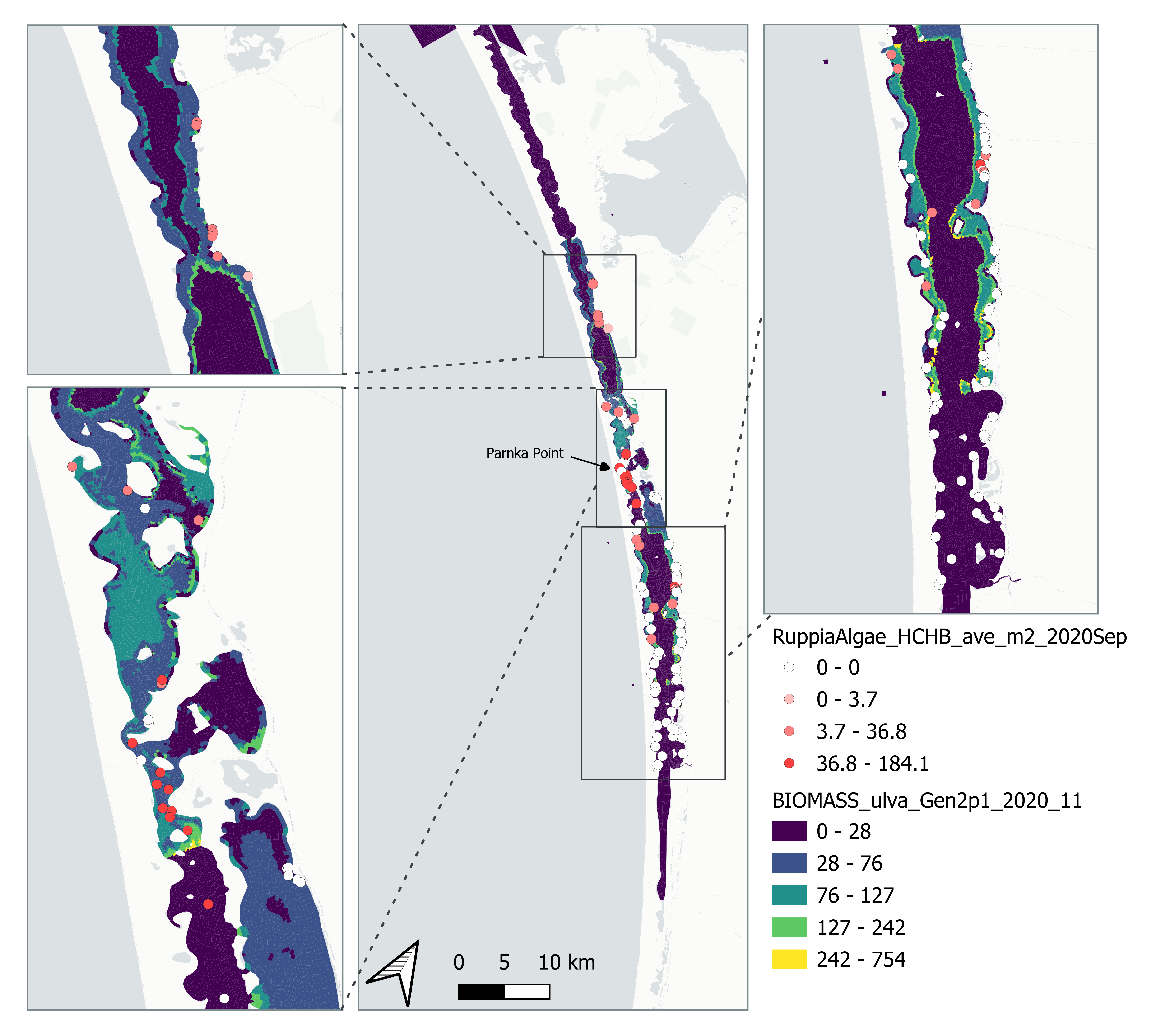
Figure 6.7: Comparison of Observed and Simulated Ulva biomass (g DW/m2) for 2020.
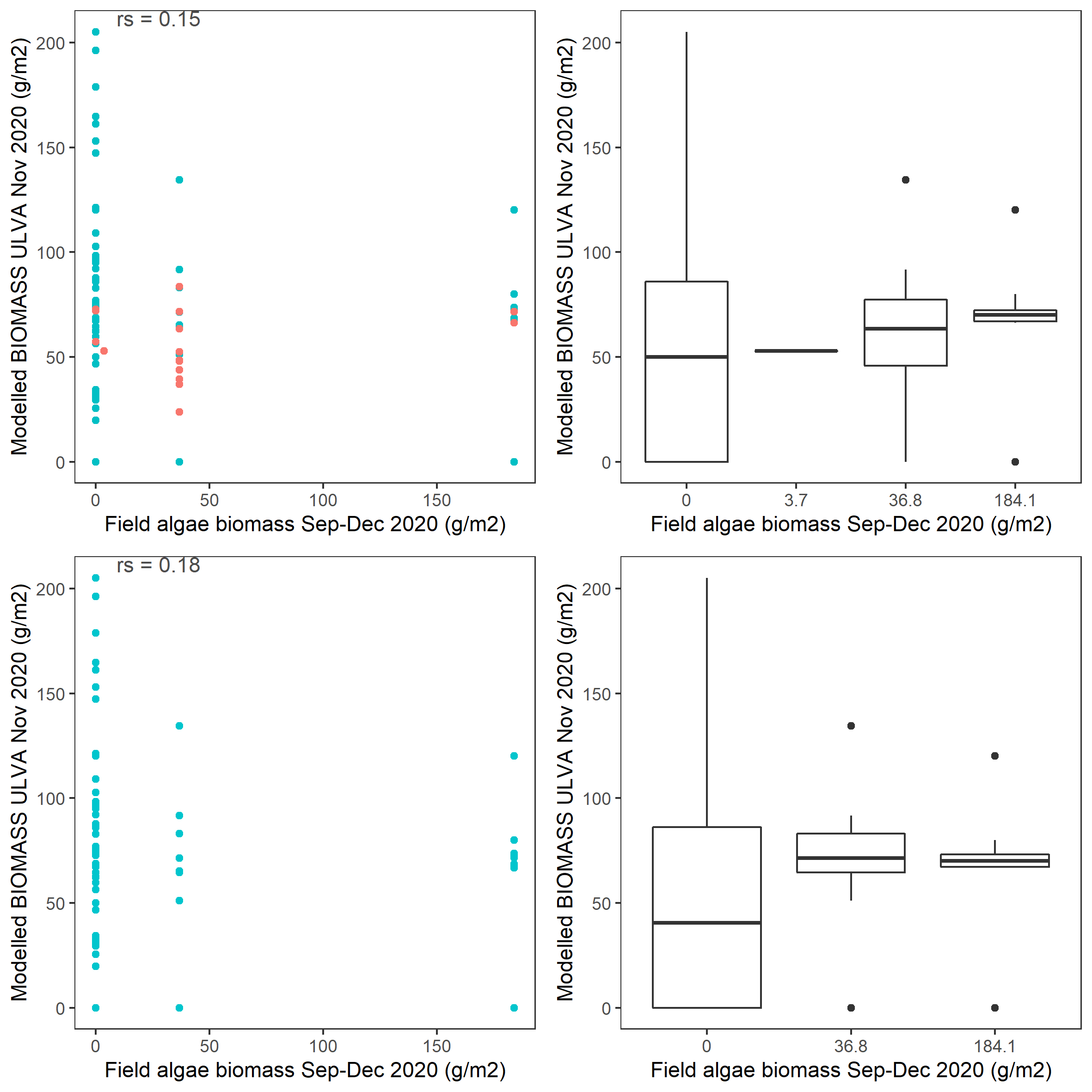
Figure 6.8: Scatter and box plot of field estimated macroalgae biomass versus simulated Ulva biomass for 2020 in the entire lagoon (top panel: red - north lagoon sites; blue - south lagoon sites) and south lagoon (bottom panel). rs: Spearman’s rank correlation coefficient.
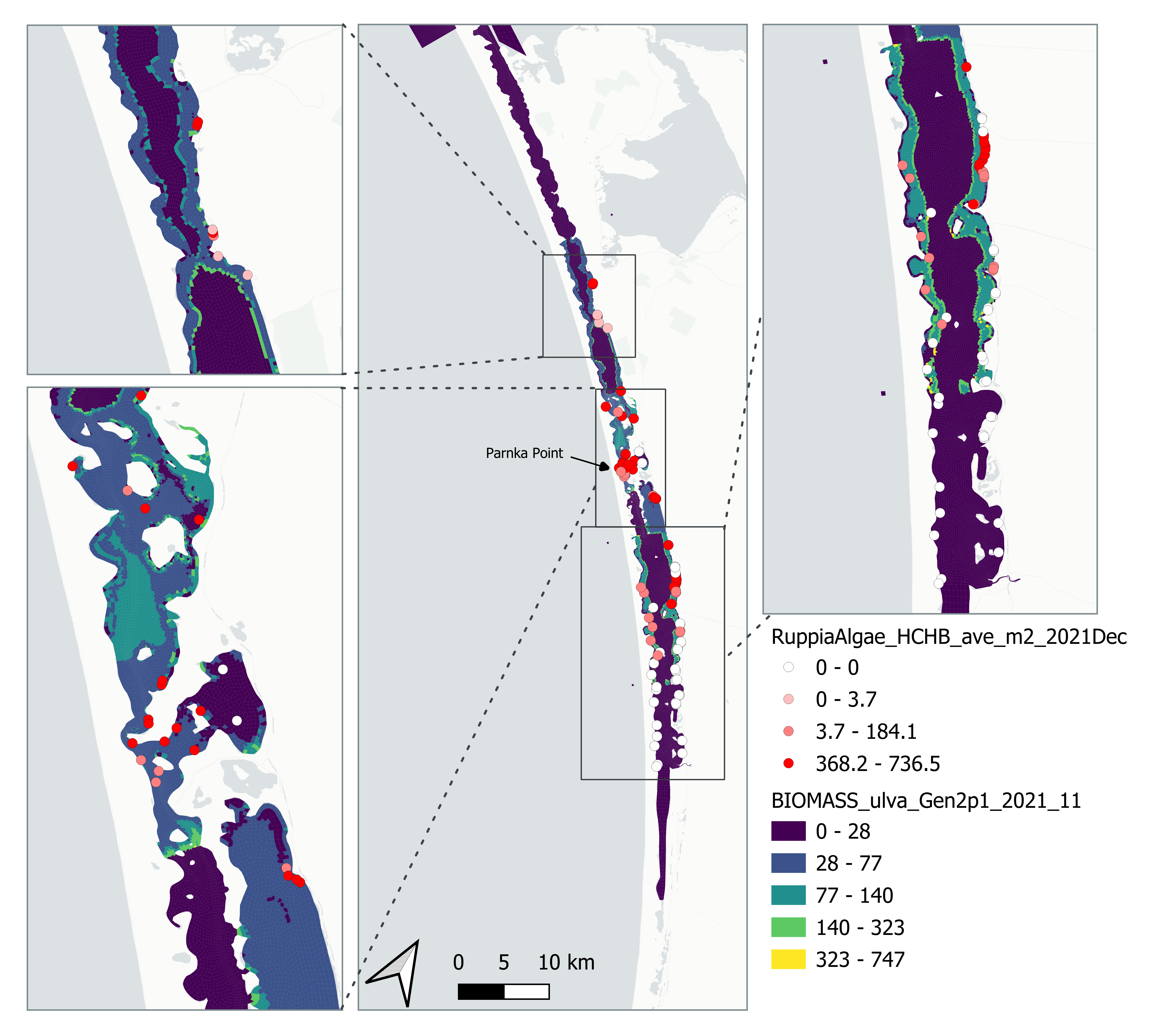
Figure 6.9: Comparison of Observed and Simulated Ulva biomass (g DW/m2) for 2021.
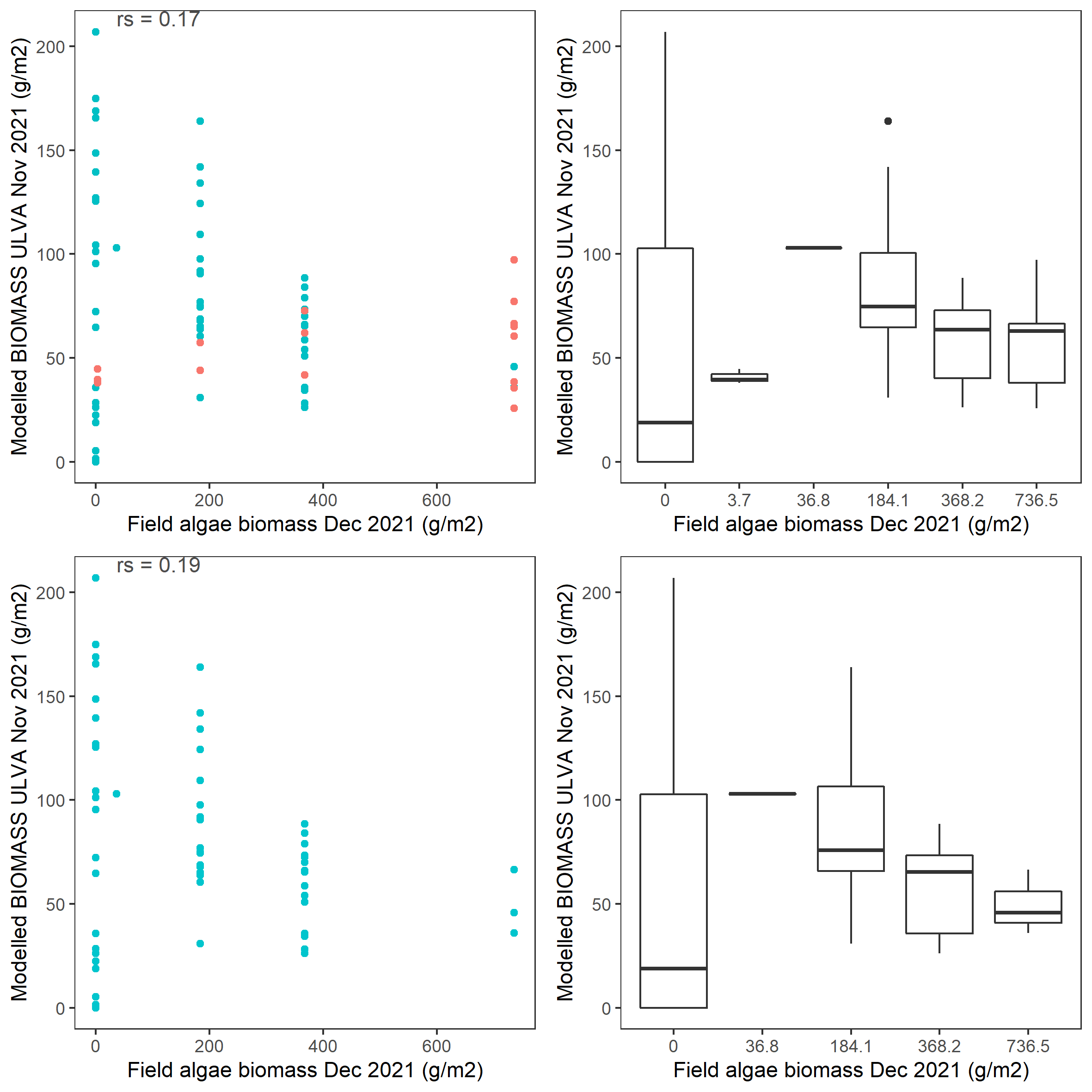
Figure 6.10: Scatter and box plot of field estimated macroalgae biomass versus simulated Ulva biomass for 2021 in the entire lagoon (top panel: red - north lagoon sites; blue - south lagoon sites) and south lagoon (bottom panel). rs: Spearman’s rank correlation coefficient.
Comparison of zone averaged modelled and observed data in 2020 - 2021 is shown in Figure 6.11.The model did capture accurately that several zones should have no or low biomass, the zones indicated by zeros in Figure 6.11. The model recorded zone-averaged biomass accumulating in some zones where observed biomass was lower (e.g. zone 31,33). Therefore, the model isn’t capturing the spatial gradient as seen in the field data.
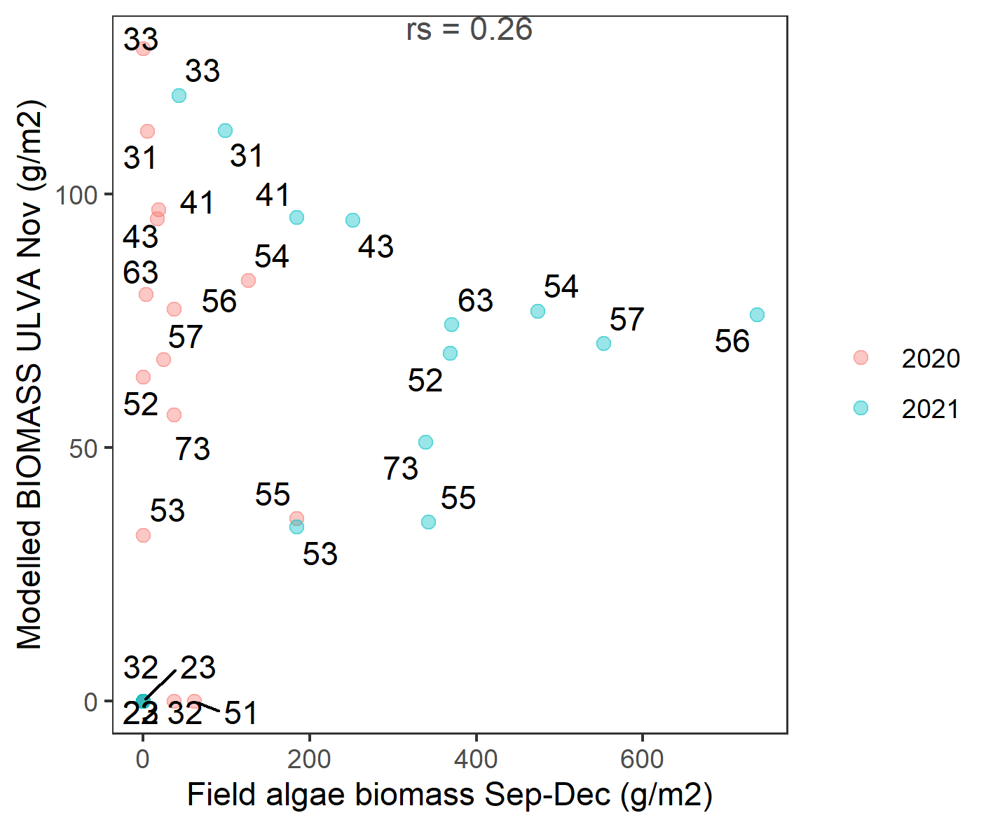
Figure 6.11: Scatter plot of field estimated macroalgae biomass versus simulated Ulva biomass for 2020 - 2021 averaged by zones in the lagoon. Labels indicate zone number (see Figure 2.5 for details). rs: Spearman’s rank correlation coefficient.
Closer inspection of the controls on growth are highlighted in the animation below.
6.6 Summary
The macroalgae model in AED has been able to capture the broad spatial patterns in environmental drivers that control the drivers and biomass of the Ulva community. Comparison of the Generation 0 model with the pre-HCHB survey data provided insights to the suitability of the model approach, and demonstrated the growth drivers (as captured via the \(Ulva\:HSI\)) correlated well with the early (albeit patchy) observations of biomass occurrence. This has been further refined in the Generation 1, 1.5 and 2.0 model simulations to ultimately allow simulation of the spatial extent of filamentous algal biomass accumulation.
The Generation 2.1 model showed mixed accuracy against the more comprehensive dataset from 2020 and 2021 with a more notable number of false positives - areas where biomass was predicted to occur but was not observed in the field. This is recommended as an area for further investigation and may benefit from further data on benthic substrates that can be used to constrain where it is able to attach and grow.