5 Oxygen, Nutrients & Chlorophyll-a

5.1 Overview

Coastal lagoons occur along 13% of the coastlines of all continents (Barnes, 1980) and represent a special type of coastal systems in terms of their hydrology and biogeochemistry, where strong gradients in chemical variables and ecosystem function persist (Kjerfve, 1994). Coastal lagoons like the Coorong are shallow with restricted connection with the ocean, and become vulnerable to nutrient enrichment and eutrophication. Choked lagoons have comparatively long water retention time and high phytoplankton biomass (Knoppers et al., 1991; Newton and Mudge, 2005) due to the restricted water exchange. The relatively poor flushing, together with shallow bathymetry and evaporation, leads to accumulation of salt and nutrients within the basins that is not easily flushed out. Within the South Lagoon in particular, the intense cycling of N and P between the organic and inorganic forms is mediated by the many complex controls on oxygen solubility and primary productivity.

Furthermore, the biogeochemical cycle of hypersaline environments is highly distinct from typical freshwater, estuarine or marine environments because it is strongly affected by changes in the physicochemical parameters of the brine as well as in the state and composition of the biological community in response to the salinity variations (Isaji et al., 2019; Mosley et al., 2020; Zhang and Huang, 2011). The use of water quality models in the management of coastal water has been well recognised and many models have been utilized to date for coastal management, however, water quality models considering hypersaline lagoon environments are relatively rare although extensive hydrodynamic modelling has been undertaken in these systems.

Therefore, whilst the base AED model platform being used in previous model versions has been a good starting point, there is a need to tailor the setup to the hypersaline Coorong lagoon system. The aim of this section is to describe the approach, model adjustments and model assessment in terms of how the model is applied to capture the core biogeochemical components: the oxygen, nutrients, and phytoplankton that form the foundation of the elemental cycles in the lagoon.

5.2 Dissolved Oxygen

5.2.1 Background

Dissolved Oxygen (\(DO\)) dynamics respond to processes of atmospheric exchange, sediment oxygen demand, microbial use during organic matter mineralisation and nitrification, photosynthetic oxygen production and respiratory oxygen consumption, chemical oxygen demand and respiration by other biotic components. In general, within the Coorong, dissolved oxygen levels are affected by salinity and temperature changes, which control oxygen solubility. In the South Lagoon however, enriched sediments create a large sediment oxygen demand (\(SOD\)), which can casue a temporary sag in the oxygen saturation levels, particualr under quiescent conditions when wind mixing is unable to replenish low oxugen in the bottom waters. Superimposed on this is the often patchy photosynthetic inputs of oxygen by phytoplankton and filamentous macroalgae, and their subsequent high respiratory demands under dark conditions.

5.2.2 Model setup

The CDM oxygen modelling approach follows the AED oxygen model setup as outlined in the AED science manual. The configuration used in the CDM simulations includes:

• atmospheric exchange, based on oxygen solubility
• phytoplankton photosynthesis and respiration
• microphytobenthos photosynthesis and respiration
• macroalgae photosynthesis and respiration
• sediment oxygen demand
• oxygen consumption due to nitrification
• oxygen consumption due to organic matter mineralisation

The sediment oxygen demand is calculated either by the static sediment oxygen model, or when the SDG model is engaged, then the sediment oxygen demand is computed dynamically based on the oxygen gradient across the sediment-water interface.

The settings for the model run with the static sediement oxygen demand models, include sensitivity of the SOD to temperature and oxygen concentration in the overlying water. The base oxygen flux rate is however specified for each sediment zone; this is summarised in more detail in the subsequent section.

Aside from the sediment oxygen demand, the parameters used in the oxygen module are largely fixed and based on either the solubility constants for oxygen, and the reaction rates computed in the nutrient and primary producer modules based on a pre-determined oxygen stoichiometry.

5.2.3 Model results

The oxygen predictions have been assessed over various years of conditions in the Coorong (2017-2021) based on the routine oxygen monitoring data available, in addition to the once-off high-frequency oxygen logger deployment undertaken at McGrath. In assessing the model performance, we sought to ensure:

• the mean solubility condition across the lagoon was resolved along the salinity gradient
• the seasonal cycle of solubility was reproduced in the mouth, south lagoon and north lagoon
• the high-frequency measurements of diel oxygen variation were resolved in the deep (open) water monitoring sites, and
• the high-frequency measurements of diel oxygen variation were resolved in the shallow (littoral) water monitoring locations, which have higher densities of macrophytes and macroalgae.

The results of the integrated assessment for the final calibrated model are shown in Chapter 9, and below some focused results are presented to demonstrate model performance in simulation oxygen dynamics.

Oxygen metabolism at McGrath

Figure 5.1 shows the modelled dissolved oxygen saturation levels against the high frequency oxygen logger data that was collected at the site of McGrath. The results indicate the model captures diel oxygen metabolism at this site well, with fluctuations of high oxygen saturation levels in the day time and low oxygen saturation level at the night time, due to primary production and respiration, respectively.

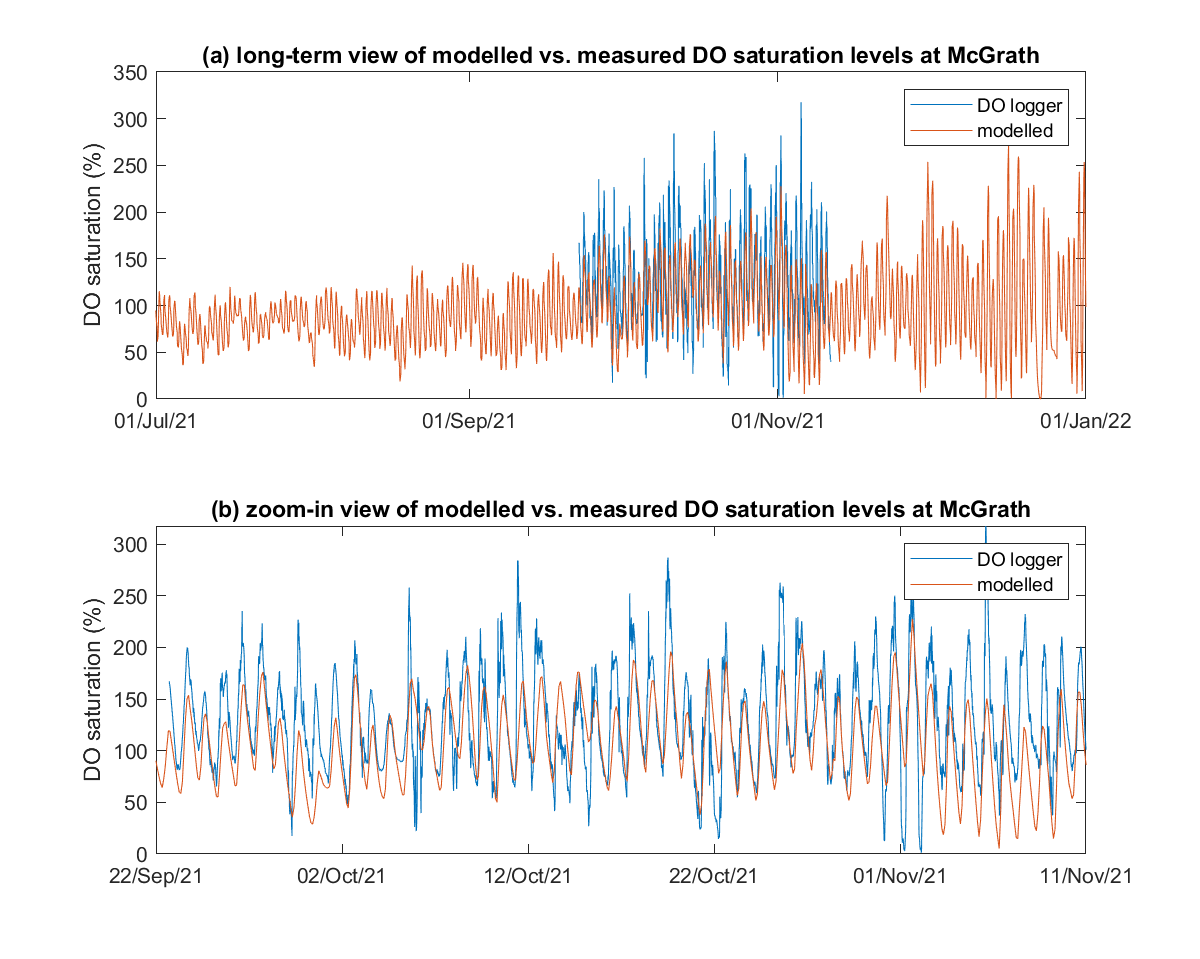
Figure 5.1: (a) Long-term time-series and (b) zoom-in view of the modelled vs. measured DO saturation levels at McGrath.

Long-term oxygen predictions

The predictions of oxygen concentrations for the main calibration (2020-2021) and validation (2017-2021) multi-year assessments are shown in Appendix B : Results Archive.

5.3 Nitrogen, Phosphorus & Silica

5.3.1 Background

Nutrient retention in the Coorong lagoon is currently a core management driver, linked to habitat quality and a key target of proposed management interventions. Recent analysis of the available historical nutrient data across the lagoon has shown the sharp gradients in nutrient species, and often high levels of nutrients in the South Lagoon in particular (Mosley et al., 2021). Furthermore, process investigations have elucidated the high rates of benthic metabolism and rates of productivity, contributing to a system with intensively cycled materials between ecosystem pools. Yet, we currently have only a limited understanding of the nutrient budget within the lagoons and the hydrodynamic and biogeochemical controls on elemental cycling. In this section, we outline the model setup and approach to parameterisation and parameter selection for the key pools and processes relevant to the Coorong.

5.3.2 Model setup

General approach

The CDM approach to simulate nutrients includes the nitrogen, phosphorus, silica and organic matter modules within AED. Both the inorganic and organic, and dissolved and particulate forms of C, N and P are modelled explicitly along the general degradation pathway of POM to DOM to dissolved inorganic matter (DIM), however the need for discrete OM pools is elaborated upon below. The nitrogen cycle includes the additional processes of denitrification and nitrification that are not in the carbon and phosphorus cycles.

An 8-pool organic matter module able to capture the variable reactivity of the OM pool and its stoichiometry is included. Under this conceptual model the decomposition of particulate detrital material is broken down through a process of enzymatic hydrolysis that slowly converts POM to labile DOM. A small fraction, f_ref, of this material is diverted to the DOM-R pool. The bioavailable DOM material enters the bacterial terminal metabolism pathways. These are active depending on the ambient oxygen concentrations and presence of electron acceptors, and of most relevance to the reservoirs, these pathways aerobic breakdown, denitrification, sulfate reduction, and methanogenesis. In most model approaches it is assumed these communities vary in response to temperature, and are mediated using a simple oxygen dependence or limitation factor. Reoxidation of reduced by-products is also included to account the role of nitrifiers, sulfate oxidising bacteria (SOB) and methane oxidising bacteria (MOB).

Filterable reactive phosphorus also is known to adsorb onto suspended solids (SS), however, the rate is often site specific. Particulate organic matter in that deposits into the sediment may also be resuspended back into the water column when the bottom shear stress is adequate. In addition to the normal process descriptions included in the AED modules summarised above, several adjustments were made during the Coorong application, as dsicussed next.

Impact of hypersalinity on nitrification and denitrification

The hypersalinity in the Coorong also has potential to impair the nitrification-denitrification process which is regarded as a function to remove the nitrogen in healthy coastal wetland systems. Multiple studies have suggested that the nitrification and denitrification rates in estuarine environments generally decrease with increasing salinity (Enrich-Prast et al., 2015; Helder and De Vries, 1983; Isaji et al., 2019). Salinity inhibits ammonia oxidizing bacteria activity that has been observed to lead to enrichment of ammonium with salinity (Cui et al., 2016; Isaji et al., 2019). This is coincident with the finding in the Coorong that strong ammonium flux from sediment and high ammonium concentrations within surface sediments observed at Parnka Point (Mosley et al., 2020). In the Coorong, it also has been found that the denitrification gene nirK had a strong inverse relationship with salinity, and the decline of the nirK concentration became more significant when the salinity was over about 40 PSU (Mosley et al., 2020). Therefore, a Michaelis-Menten kinetic function of salinity limitation has been adopted for the nitrification and denitrification rates within the water columns as:

\[\begin{equation} f_{SAL}=\begin{cases} 1, & \text{when $S \le S_{thresh}$}\\ \frac{K_S}{K_S+(S-S_{thresh})}, & \text{when $S>S_{thresh}$} \end{cases} \end{equation}\]

where \(f_{SAL}\) is the limitation factor, \(S\) the salinity, \(S_{thresh}\) the salinity threshold when limitation starts to work, and \(K_S\) is the half saturation coefficient. In the Coorong, the \(S_{thresh}\) is set to 40 PSU and \(K_S\) is set to 20 PSU as interpolated from the report of Mosley et al. (2020). This is shown graphically in Figure 5.2.

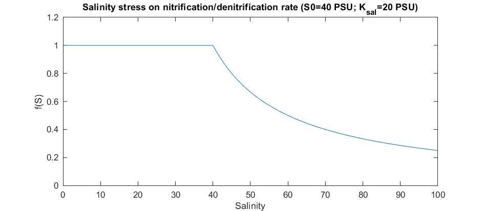
Figure 5.2: Limitation factor of salinity on base nitrification and denitrification rates.

Impact of salinity and temperature on phosphorus adsorption-desorption

Because of low solubility of P-bearing minerals in the earth’s crust and a strong affinity of dissolved phosphate to adsorb on the solid surfaces, sediment, including suspended particles, has been identified as the dominant P reservoir in both freshwater and coastal marine environments. Suspended particles are able to adsorb or desorb phosphate in the water, depending on the sediment phosphorus contents and a range of environmental conditions. Adsorption can vary considerably along a salinity gradient (Sundareshwar and Morris, 1999; Zhang and Huang, 2011) as well as affected by the temperature (Zhang and Huang, 2011). For this process adoption of the algorithm, as implemented by Zhang and Huang (2011), is a convenient method. In this method, the PO4 adsorption capability (\(K_{PO4-P}\)), defined as the ratio of \(PO_4\) concentration in the particles and water per mg of suspended particles, is calculated as:

\[\begin{equation} K_{PO4-P} = (60- [EPC]_0)/(100 ×[EPC]_0) \tag{5.1} \end{equation}\]

where the \([EPC]_0\) is the equilibrium \(PO_4\) concentration in the water and is a function of the exchangeable \(PO_4\) content in the particle \(P_{exch}\), calculated as:

\[\begin{equation} [EPC]_0 = A × P_{exch} +B×P_{exch}^2 \tag{5.2} \end{equation}\]

where \(A\) and \(B\) in Eq (5.2) are coefficients as a function of salinity and temperature through multi-parameter regression analysis from laboratory experiments as:

\[\begin{equation} A=-140.5+1098.2/T+30.67× ln(T)+0.0907×S \\ B=1225.96-6880.49/T-278.77×ln(T))+0.4561×S \tag{5.3} \end{equation}\]

where \(T\) is the water temperature in °C, \(S\) is the salinity in PSU. In the Coorong, the \(P_{exch}\) is estimated as 0.78 µmol P/g from the field survey data (Mosley et al., 2020). The resulting \(PO4\) adsorption capability under a range of temperature and salinity is shown graphically in Figure 5.3.

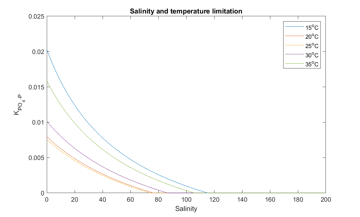
Figure 5.3: Response of the adsorption capability of phosphorus of suspended particles to water temperature and salinity.

Nutrient flux at the sediment-water interface (SWI)

One of the key drivers of lagoon water quality is the sediment biogeochemical processes and the exchange of nutrient at the SWI (Crowe et al., 2012). In shallow waters, hydrodynamics and diffusion have been regarded as the crucial factors to dominate the rate of sediment nutrient release. More specifically, two modes are responsible for nutrient release from sediment layers to overlying water: static release by nutrient diffusion in relatively calm situations as driven by a concentration gradient, and dynamic release accompanied by hydrodynamic-induced sediment resuspension (Qin et al., 2006; Tengberg et al., 2003). In open water where the fetch is long, in particular, the dynamic release can be the dominant mode since the water-sediment interface is frequently disturbed by hydrodynamic processes (Qin et al., 2006). Fan et al. (2001) have claimed that the internal phosphorus (P) load induced by resuspension was 8–10 times larger than the static release, while Reddy et al. (1996) have reported that ammonia concentration increased ten times in the overlying water caused by resuspension compared with gradient diffusion. It is also found that internal P from sediment resuspension resulting from moderate wind could be comparable in magnitude to the daily external supply Gelencser et al. (1982). Thus, the disturbance at the water-sediment layer induced by wind can significantly affect SS and nutrient behaviors in shallow aquatic ecosystems (Huang et al., 2016).

Resuspension leads to a predictable increase of suspended solids (including POC) in the overlying water, but the impacts on the dissolved nutrient release rate depends on many factors. Tengberg et al. (2003) showed the resuspension led to an increase flux of NO3, but decrease of PO4 and no change of NH4. Similarly, Tengberg et al. (2003) and Sondergaard et al. (1992) found that resuspension can led to either higher or lower concentration of phosphate in the overlying water, depending the iron level of the suspended solids. Furthermore, the effects of resuspension on the long-term nitrogen and phosphorus liberation may be mild. (Sloth et al., 1996) showed small changes in nutrient fluxes in the laboratory study, and the measured parameters of a marine system returned to the condition before the resuspension events. Blackburn (1997) also stated that natural resuspension does not significantly contribute to a long-term change of sediment nitrogen release. The nitrogen release with or without resuspension is just a matter of time, that is a sudden or a gradual release but to the same extent.

In the Coorong, the effects of wind-induced resuspension on the nutrient release in the Coorong may be relatively mild. In the field survey of waves and resuspension in the Coorong, there was no significant change in nutrient levels due to resuspension. Total nutrient concentrations did not show a consistent relationship to any other variables and TN and TP had a moderately negative relationship to each other. Dissolved nutrient concentrations were consistently below minimum detectable levels. This is probably due to the major components of N/P released by resuspension was the particulate forms (Tang et al., 2020); also, the sediment experiment showed a strong diffusive nutrient flux of NH4 and PO4 under calm condition, which indicate the diffusive flux of nutrient is the major process of sediment release in the Coorong. The major components of TSS in the Coorong was found to be phytoplankton, where the inorganic suspended particles contributed relatively small to the TSS.

Therefore, in the CDM generation one the “static” sediment flux algorithm is adopted that is suited to long-term studies and assumed the OM concentration is thought to be relatively stable. The sediment oxygen demand and nutrient flux rates were set based on the sediment flux data from the site of Parnka Point (Table 5.1) which were then interpolated into the zones based on the sediment particle sizes and organic matter contents, following a role of thumb that the oxygen demand and nutrient flux increased with the organic matter contents (Table 5.2).

Table 5.1: Summary of dissolved sediment flux data collected within the Coorong (HCHB T&I 1) and used in the CDM model.

Dataset	Units	Light	Dark
SWI ammonium flux
Mosley et al. (2020)	\[\mu mol\: /m^2\: /h\]	253 ± 88.4	172.5 ± 107.6
AED, Fsed_amm	\[mmol\:/ m^2\:/d\]	6.07 ± 2.12	4.14 ± 2.58
SWI nitrate flux
Mosley et al. (2020)	\[\mu mol\: /m^2\: /h\]	267.2 ± 269.8	2.90 ± 43.6
AED, Fsed_nit	\[mmol\:/ m^2\:/d\]	6.41 ± 6.47	0.07 ± 1.05
SWI phosphate flux
Mosley et al. (2020)	\[\mu mol\: /m^2\: /h\]	5.6 ± 5.8	28.3 ± 16.9
AED, Fsed_frp	\[mmol\:/ m^2\:/d\]	0.13 ± 0.14	0.68 ± 0.41
SWI oxygen flux
Mosley et al. (2020)	\[\mu mol\: /m^2\: /h\]	1546 ± 2857	-4925 ± 541
AED, Fsed_oxy	\[mmol\:/ m^2\:/d\]	37.1 ± 68.57	-118.2 ± 12.98

These sediment flux parameters serve as the default values used in the intial simulations. When the model is run with the dynamic sediment biogeochemistry model this fluxes in the tables are not used as input parameters, but rather as guides for validation of the predicted rates - see Chapter 7 for further detail about the dynamic prediction of sediment nutrient fluxes.

Table 5.2: Summary of sediment oxygen demand and nutrient fluxes setting in the CDM with 31 material zones.

Description	Zone ID	Oxygen flux (SOD)	Ammonium flux	Nitrate flux	Phosphate flux
Ocean Side	Zone 11	-8.40	7.7040	-0.0057	0.12313
Channel	Zone 12	-103.20	13.3920	-0.0136	0.68013
Lakes Side	Zone 13	-8.40	7.7040	-0.0057	0.12313
Ocean Side	Zone 21	-6.24	7.5744	-0.0055	0.11272
Channel	Zone 22	-103.20	13.3920	-0.0136	0.68013
Lakes Side	Zone 23	-8.40	7.7040	-0.0057	0.12313
Ocean Side	Zone 31	-47.88	10.0728	-0.0090	0.31345
Channel	Zone 32	-87.60	12.4560	-0.0123	0.90492
Lakes Side	Zone 33	-8.40	7.7040	-0.0057	0.72313
Ocean Side	Zone 41	-0.24	7.2144	-0.0050	0.08380
Channel	Zone 42	-117.60	14.2560	-0.0148	0.64954
Lakes Side	Zone 43	-0.24	7.2144	-0.0050	0.08380
Ocean Side	Zone 51	-55.80	7.0320	-0.0097	0.35163
Channel	Zone 52	-117.60	9.5040	-0.0148	0.64954
Lakes Side	Zone 53	-12.00	5.2800	-0.0060	0.41319
Ocean Side	Zone 61	-6.60	5.0640	-0.0056	0.11445
Channel	Zone 62	-113.52	9.3408	-0.0145	0.62987
Lakes Side	Zone 63	-6.60	5.0640	-0.0056	0.11445
Ocean Side	Zone 71	-6.60	5.0640	-0.0056	0.08900
Channel	Zone 72	-22.20	5.6880	-0.0069	0.14751
Lakes Side	Zone 73	-6.60	5.0640	-0.0056	0.08900
Ocean Side	Zone 81	-6.60	5.0640	-0.0056	0.08900
Channel	Zone 82	-60.24	7.2096	-0.0100	0.16440
Lakes Side	Zone 83	-6.60	5.0640	-0.0056	0.08900
Ocean Side	Zone 91	-0.12	4.8048	-0.0050	0.06471
Channel	Zone 92	-60.24	7.2096	-0.0100	0.09644
Lakes Side	Zone 93	-0.12	4.8048	-0.0050	0.06471
Ocean Side	Zone 101	-2.04	4.8816	-0.0052	0.07190
Channel	Zone 102	-13.68	5.3472	-0.0061	0.11553
Lakes Side	Zone 103	-2.04	4.8816	-0.0052	0.07190
Ocean Fan	Zone 104	0.00	4.8000	-0.0050	0.06429

Parameter summary

A summary of the overall model parameters used within the CDM simulations related to nutrient dynamics are summarised below in Table X.

5.3.3 Model results

A summary of the model performance for several nutrient variables is shown in Figure 5.4, for a wet and dry period in 2018-2019. The results show the gradient along the lagoon, and also the very low concentrations of bio-available nutrient fractions within the total pool. Further results of the nutrient variables are reported in the integrated assessment of the model in Chapter 9. The predictions of nutrient concentrations for the main calibration (2020-2021) and validation (2017-2021) multi-year assessments are shown in Appendix B : Results Archive. Appendix B also includes the results of a sensitivity analysis undertaken to assess the relative importance of sediment nutrient flux rates on the overlying water nutrient and chlorophyll-a concentrations.

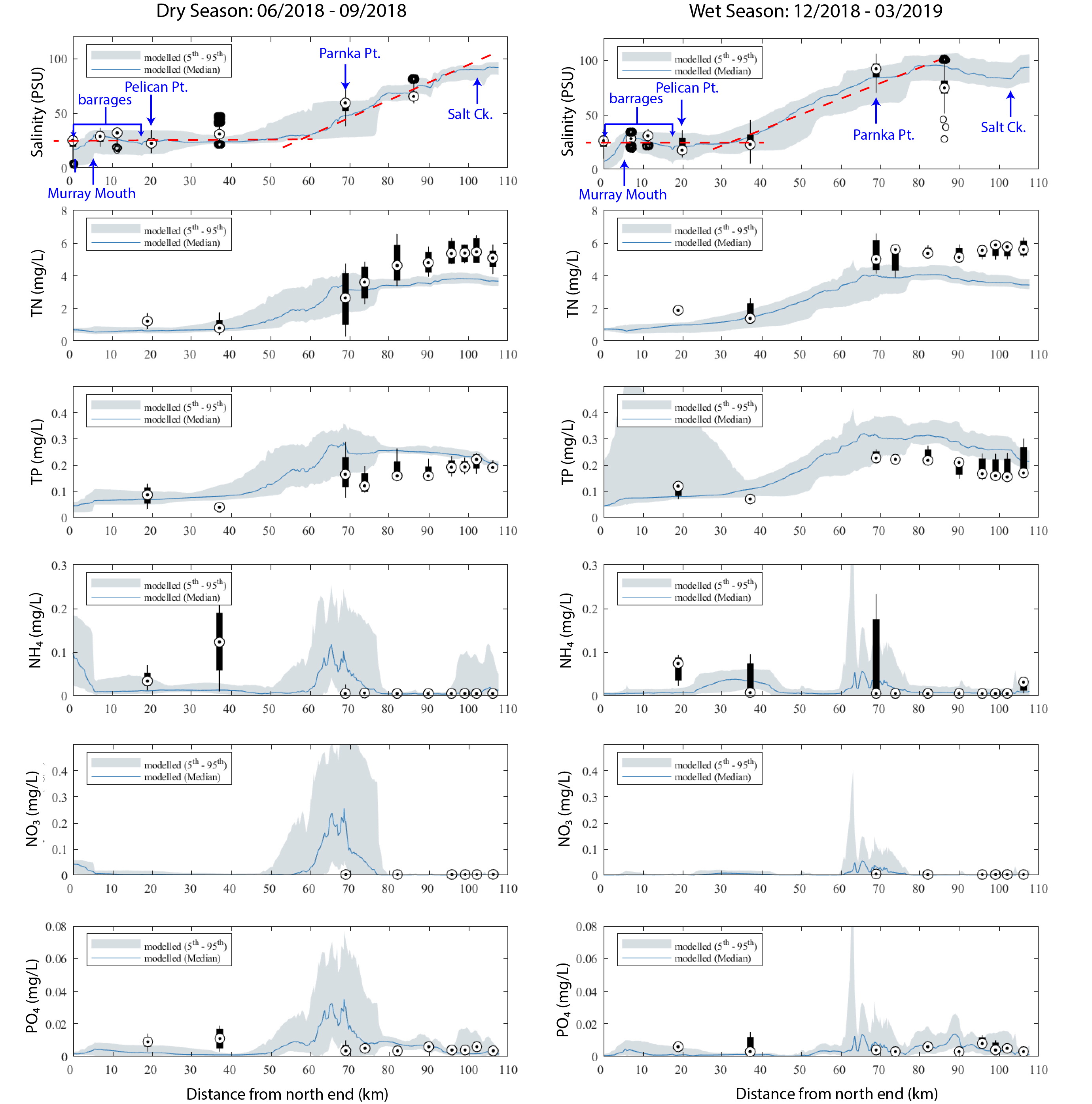
Figure 5.4: Performance of predicted nutrient concentrations along the length of the Coorong. The observed (field) data is from available monitoring over the period of a dry season (left) and wet season (right), presented as a box-whisker plot for each site based on all data available for that site within that period.

5.4 Phytoplankton & Chlorophyll-a

5.4.1 Background

Within the Coorong, salinity has been identified as the most important driver of the phytoplankton community (Jendyk et al., 2014; Leterme et al., 2015; Schapira et al., 2010). The water in the north lagoon is brackish because of mixing between the ocean and barrage flows, and this area is generally dominated by chlorophytes since the salinity threshold for dominant chlorophyte species in the lagoon is reported to be ~28 PSU. On the other hand, the water in the south lagoon is hypersaline and generally dominated by diatoms. Cryptophytes and dinoflagellates have also be documented throughout both lagoons but in comparatively lower abundance and biomass (Jendyk et al., 2014; Leterme et al., 2015).

More specifically, this paper proposed 4 salinity regimes that tend to shape phytoplankton habitat:

• waters in the H1 category (<5 PSU) which tend to be dominated by chlorophytes, although diatoms and cryptophytes sporadically accounted for between 10 and 50% of the overall phytoplankton abundance at Site 1 and Site 2.
• waters in the H2 category (5–20 PSU) are co-dominated by chlorophytes, diatoms and cryptophytes with no significant temporal differences in the relative overall abundance evident.
• waters in the H3 category (21–40 PSU) saw a drastic decrease in the prevalence of chlorophytes compared to lower salinity habitats, and a marked increases in the abundance of dinoflagellates, particularly toward the higher end of the salinity spectrum.
• waters the H4 category (>41 PSU) which are mainly dominated by diatoms, although the abundance of dinoflagellates was sometimes higher than that of diatoms.

Aside from these main habitat-species groupings, Schapira et al. (2010) had previously reported on the Coorong phytoplankton community. The major conclusions from theri study were:

• salinity was identified as the main factor structuring the distribution of pico-phytoplankton along the lagoon;
• the highest pico-phytoplankton abundances were recorded under salinity conditions ranging between 8.0% and 11.0%;
• one population of pico-eukaryote dominated the community throughout the salinity gradient and was responsible for the bloom observed between 8.0% and 11.0%. Only this halotolerant population and Prochlorococcus-like pico-cyanobacteria were identified in hypersaline waters (i.e. above 14.0%).

In addition to the phytoplankton assemblage (algae and cyanobacteria suspended in the water), the lagoon is also characterised by benthic microalgae - the so-called microphytobenthos (MPB). These have been shown to vary along the lagoon as part of the The Living Murray ecological sampling (Dittman et al., 2021). As with the phytoplankton biomass, the benthic chlorophyll-a biomass is also controlled by the sharp salinity gradient with significantly higher biomass in the North Lagoon.

The subsequent sections document the phytoplankton (\(PHY\)) and microphytobenthos (\(MPB\)) modelling approach and rationale, and the results and analysis, with comaprisons against available chlorophyll-a data within the lagoon.

5.4.2 Model setup: Phytoplankton

The approach to simulate algal biomass is to adopt several plankton functional types (PFTs) that are typically defined based on specific groups. Whilst each group that is simulated is unique, they share a common mathematical approach and each simulate growth, death and sedimentation processes, and customisable internal nitrogen, phosphorus and/or silica stores. Distinction between groups is made by adoption of group’s specific parameters for environmental dependencies, and/or enabling options such as vertical migration or N fixation. This way the group-specific traits are used to inform the groups parameterisations.

Based on the findings of the above-cited studies, the phytoplankton community in the CDM has been configured into four PFTs, according to their salinity tolerance and literature review of their biogeochemical properties asscoiated with the dominant taxa - spanning green algae (chlorophytes), cryptophytes, dinoflagellates, and diatoms.

The algal biomass of each group, \(PHY_C\), is simulated in units of carbon (\(mmol\:C/m^3\)), and the groups have been configured to have a constant C:N:P:Si ratio (this can be alternatuvely changed to use dynamic stoichiometry and uptake of N and P sources in response to changing water column condition and cellular physiology if preferred). The total water column chlorophyll-a is calculated from the sum of the individual groups with a carbon:chlorophyll-a conversion applied. Balance equations that capture the various processes impacting phytoplankton are outlined in the full description of the phytoplankton model within the AED science manual. Key aspects relevant to the Coorong implementation are summarised in the following sections, including the salinity limitation functions and parameters used to differentiate the phytoplankton groups within the community.

The four pools configured to simulate the biomass of phytoplankton, were denoted \(grn\), \(crypt\), \(diatom\) and \(dino\), which map to the mixed assemblage groups identified above as \(H1\) - \(H4\). The parameters used in the setup are outlined in Table (Table 5.3).

Table 5.3: Summary of the phytoplankton parameters used in the CDM version of the AED model.

Parameter	Description	Unit	Parameter1	Parameter2	Parameter3	Parameter4
General
\[a\]	name of phytoplankton group	\[\small{-}\]	‘grn’	‘crypt’	‘diatom’	‘dino’
\[PHY |_{t=0}\]	initial concentration of phytoplankton	\[\small{mmol\: C/m^3}\]	10	10	10	10
\[PHY_0\]	minimum concentration of phytoplankton	\[\small{mmol\: C/m^3}\]	0.2	0.2	0.2	0.2
\[\chi_{C:chla}^{PHY}\]	carbon to chlorophyll ratio	\[\small{mg\: C/mg\: chla}\]	50	50	50	50
Growth
\[R_{growth}^{PHY}\]	phytoplankton group maximum growth rate at \(20^{\circ}C\)	\[\small{/d}\]	2.4	1.8	3.1	2.1
\[\Theta_{tem}^{phy}\]	specifies temperature limitation function of growth	\[\small{-}\]	1	1	1	1
\[\theta_{growth}^{phy}\]	Arrenhius temperature scaling for growth function	\[\small{-}\]	1.08	1.08	1.08	1.08
\[T_{std}\]	standard temperature	\[\small{^{\circ}C}\]	18	20	18	18
\[T_{opt}\]	optimum temperature	\[\small{^{\circ}C}\]	23	26	28	25
\[T_{max}\]	maximum temperature	\[\small{^{\circ}C}\]	35	38	39	32
Light
\[\Theta_{lgt}^{phy}\]	switch to assign the type of light response function	\[\small{-}\]	0	0	0	0
\[I_K\]	half saturation constant for light limitation of growth	\[\small{W/m^2}\]	100	100	100	100
\[K_e\]	specific attenuation coefficient	\[\small{/m/(mmol\:C/m^3)}\]	0.00408	0.0051	0.00408	0.0048
\[f_{pr}\]	fraction of primary production lost to exudation	\[\small{-}\]	0.025	0.025	0.025	0.025
Respiration
\[R_{resp}^{PHY}\]	phytoplankton respiration/metabolic loss rate at \(20^{\circ}C\)	\[\small{/d}\]	0.04	0.08	0.02	0.095
\[\theta_{resp}^{phy}\]	Arrhenius temperature scaling factor for respiration	\[\small{-}\]	1.08	1.08	1.08	1.08
\[k_{fres}\]	fraction of metabolic loss that is true respiration	\[\small{-}\]	0.1	0.1	0.1	0.1
\[k_{fdom}\]	fraction of metabolic loss that is released as DOM	\[\small{-}\]	0.3	0.3	0.3	0.3
Salinity
\[\Theta_{sal}^{phy}\]	type of salinity limitation function	\[\small{-}\]	-1	-1	-2	-3
\[S_{bep}\]	salinity limitation value at maximum salinity (\(S_{maxsp}\))	\[\small{-}\]	0.1	0.1	0.1	0.1
\[S_{maxsp}\]	maximum salinity where growth is possible	\[\small{g/kg}\]	28	60	200	90
\[S_{opt}\]	optimal salinity for growth	\[\small{g/kg}\]	10	20	60	40
Nitrogen
\[\Theta_{din}^{phy}\]	switch for the selected group to simulate \(DIN\) uptake	\[\small{-}\]	1	1	1	1
\[\Theta_{don}^{phy}\]	switch for the selected group to simulate \(DON\) uptake	\[\small{-}\]	0	0	0	0
\[\Theta_{n2}^{phy}\]	switch for the selected group to simulate \(N_2\) fixation	\[\small{-}\]	0	0	0	0
\[\Theta_{in}^{phy}\]	switch for the selected group to simulate dynamic intracellular \(N\) store	\[\small{-}\]	0	0	0	0
\[N_o\]	external \(DIN\) concentration below which uptake is 0	\[\small{mmol\: N/m^3}\]	0.02	0.071	0.02	0.071
\[K_N\]	half-saturation concentration of nitrogen	\[\small{mmol\: N/m^3}\]	1.786	2.143	1.786	2.4
\[\chi_{ncon}^{PHY}\]	constant internal nitrogen concentration	\[\small{mmol\: N/m^3}\]	0.16	0.151	0.1	0.167
\[\chi_{nmin}^{PHY}\]	minimum internal nitrogen concentration	\[\small{mmol\: N/m^3}\]	0.069	0.054	0.069	0.069
\[\chi_{nmax}^{PHY}\]	maximum internal nitrogen concentration	\[\small{mmol\: N/m^3}\]	0.18	0.054	0.18	0.206
\[R_{nuptake}^{PHY}\]	maximum nitrogen uptake rate	\[\small{mmol\: N/m^3/d\: /(mmol\: C/m^3)}\]	0.069	0.032	0.069	0.206
\[k_{nfix}\]	growth rate reduction under maximum nitrogen fixation	\[\small{-}\]	0.7	0.7	0.7	0.7
\[R_{nfix}^{PHY}\]	nitrogen fixation rate	\[\small{/d}\]	6e-04	0.00075	6e-04	6e-04
Phosphorus
\[\Theta_{dip}^{phy}\]	switch for the selected group to simulate \(DIP\) uptake	\[\small{-}\]	1	1	1	1
\[\Theta_{ip}^{phy}\]	switch for the selected group to simulate dynamic intracellular \(P\) store	\[\small{-}\]	0	0	0	0
\[P_o\]	external \(DIP\) concentration below which uptake is 0	\[\small{mmol\: P/m^3}\]	0.0064	0.0064	0.0064	0.0064
\[K_P\]	half-saturation concentration of phosphorus	\[\small{mmol\: P/m^3}\]	0.2526	0.3226	0.2426	0.36
\[\chi_{pcon}^{PHY}\]	constant internal phosphorus concentration	\[\small{mmol\: P/m^3}\]	0.002976	0.0028086	0.00186	0.0031062
\[\chi_{pmin}^{PHY}\]	minimum internal phosphorus concentration	\[\small{mmol\: P/m^3}\]	0.0015	0.0015	0.0015	0.0015
\[\chi_{pmax}^{PHY}\]	maximum internal phosphorus concentration	\[\small{mmol\: P/m^3}\]	0.0096	0.0096	0.0096	0.0096
\[R_{puptake}^{PHY}\]	maximum phosphorus uptake rate	\[\small{mmol\: P/m^3/d\: /(mmol\: C/m^3)}\]	0.0031	0.0031	0.0031	0.0031
\[\Theta_{si}^{phy}\]	switch for the selected group to simulate \(Si\) uptake	\[\small{-}\]	0	0	0	0
\[Si_o\]	external \(SiO2\) concentration below which uptake is 0	\[\small{mmol\: Si/m^3}\]	0	0	0	0
\[K_{Si}\]	half-saturation concentration of silica uptake	\[\small{mmol\: Si/m^3}\]	8	8	8	8
\[\chi_{sicon}^{PHY}\]	constant internal silica concentration	\[\small{mmol\: Si/m^3}\]	0.0171	0.0171	0.0171	0.0171
\[\omega_{phy}\]	sedimentation rate	\[\small{m/d}\]	-0.05	0	-0.1	0
\[d_{phy}\]	phytoplankton group mean cell diameter	\[\small{m}\]	0	0	0	0
\[c_1\]	rate coefficient for density increase	\[\small{kg/m^3/s}\]	0	0	0	0
\[c_3\]	minimum rate of density decrease with time	\[\small{kg/m^3/s}\]	0	0	0	0
\[f_1\]	fraction of maximum intracellular nitrogen where motility tends down towards nutrients	\[\small{-}\]	0	0	0	0
\[f_2\]	fraction of maximum intracellular nitrogen where motility tends up towards light	\[\small{-}\]	0	0	0	0

In terms of understanding the productivity of phytoplankton, for informing other rate parameters in the model, (Joint et al., 2002) studied phytoplankton along a hypersalinity gradient and found that elevated photosynthetic pigment concentrations were present in ponds of intermediate (5^11%) and high (s32%) salinity, but that rates of primary production and nutrient uptake were generally reduced at the highest salinity. For example, the maximum primary production was measured at 8% salinity and chlorophyll-specific carbon fixation also maximised at this salinity under conditions where ammonium was the dominant nitrogen source throughout the salinity gradient.

Noting that salinity impacts productivity and the observations noted in the previous section in the Coorong, the salinity tolerance effect on phytoplankton was therefore given by adopting salinity tolerance functions, \(f(S)\), depending on the group’s sensitivity to salinity. There are four options adding into the \(CDM\) based on quadratic functions that are used to define the salinity effect (Griffin et al., 2001; Robson and Hamilton, 2004):

The salinity limitation settings are included in the phytoplankton parameter table and the use of various salinity limitation options for each phytoplankton PFT are shown graphically in Figure 5.5.

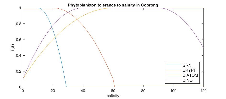
Figure 5.5: Salinity limitation curves applied to the photosynthesis rate of each phytoplankton group to acheive the phytoplankton group zonation reported in the literature.

Direct measurements for other group-specific physiological rates and parameters are not yet available for the Coorong, and so the current version of the model relies on prior experience and relevant literature to set the other key parameters shown in Table 5.3 for each group, such as the sedimentation rate, nutrient stoichiometry and light sensitivity.

---

5.4.3 Model setup: Microphytobenthos

The approach to simulate the biomass of benthic microalgae (microphytobenthos) is to allocate a single biomass pool that cocneptually sites between the water and sediment (i.e., at the sediment-water interface). The biomass of this group, \(MPB\), is simulated in units of carbon (\(mmol\:C/m^2\)), and has a dynamic C:N:P stoichiometry based on the history of the deposited phytopalnkton that have landed on the sediment. The model is conceptually simple compared to the overlying phytoplankton group model, with paramaetrs to mediate response to light, resuspension back into the watre column, and burial into the deeper sediment.Balance equations that capture the various processes impacting phytoplankton are outlined in the full description of the phytoplankton model within the AED science manual.

The \(MPB\) pool configured to simulate the biomass is configured according to the parameters outlined in Table (Table 5.4).

Table 5.4: Summary of the microphytobenthos parameters used in the CDM version of the AED model.

Parameter	Description	Unit	Parameter1
Microphytobenthos
\[R_{mpb-g}\]	maximum growth rate of \(MPB\)	\[\small{/d}\]	0.6
\[R_{mpb-r}\]	dark respiration rate of \(MPB\)	\[\small{/d}\]	0.2
\[R_{mpb-b}\]	rate of MPB burial	\[\small{/d}\]	0.2
\[I_{K_{mpb}}\]	half saturation constant for light limitation of growth	\[\small{W/m^2}\]	10
\[MPB_{max}\]	maximum biomass density of \(MPB\)	\[\small{mmol\: C/m^2}\]	1500
\[\Theta_{resus}^{phy}\]	fraction to set the amount of resuspension for \(PHY\) group \(a\)	\[\small{-}\]	1.2
\[N_{sz}^{mpb}\]	number of benthic zones where \(MPB\) is active	\[\small{-}\]	20
\[\mathbb{Z}_{sz}^{mpb}\]	set of benthic zones with \(MPB\) active, where \(sz \in \mathbb{Z}\)	\[\small{-}\]	…

5.4.4 Model results

The simulated phytoplankton biomass has been compared against the available chlorophyll-a data from the routine WQ monitoring sites. The model captures well the long-term mean gradient in biomass along the length of the Coorong, which includes the separation of the groups based on their optimum salinity and nutrient parameters (Figure 5.6).

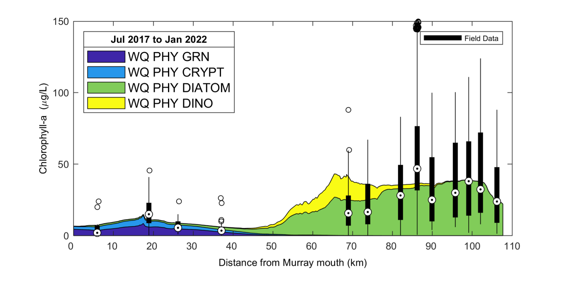
Figure 5.6: Simulated and observed chlorophyll-a concentration along the length of the Coorong from the Murray Mouth. The observed (field) data is from available monitoring over the period from Jul 2017 to Jan 2022, presented as a box-whisker plot for each site based on all data available for that site. The simulated data is shaded based on the PFT (group) contribution to the total phytoplankton biomass.

Whilst the above plot shows the along-lagoon gradient, the seasonal and high frequency variability of chlorophyll-a can be more variable and is also well-captured by the model (Figure 5.7).

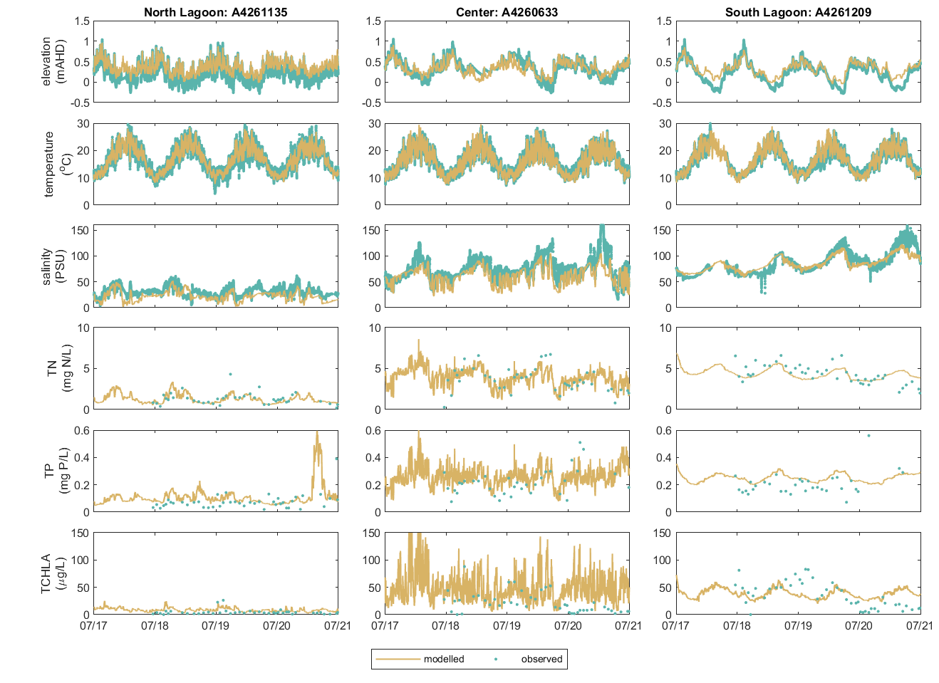
Figure 5.7: Performance of predicted phytoplankton biomass and other key water quality variables at north lagoon, center, and south lagoon.

The limitation plots for each simulated group provide insights into the dynamic environmental controls on group productivity (Figures 5.8-5.14).

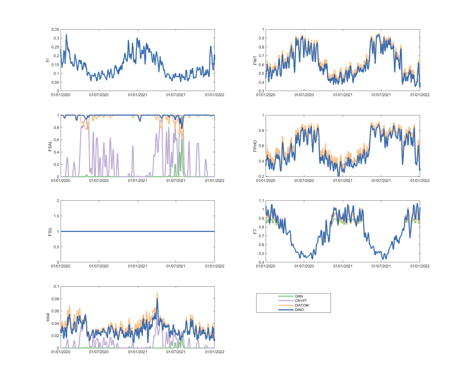
Figure 5.8: Phytoplankton environmental limitation controlling the photosynthesis rate of each phytoplankton group, for site A4260633 (Click the station ID above to change image).

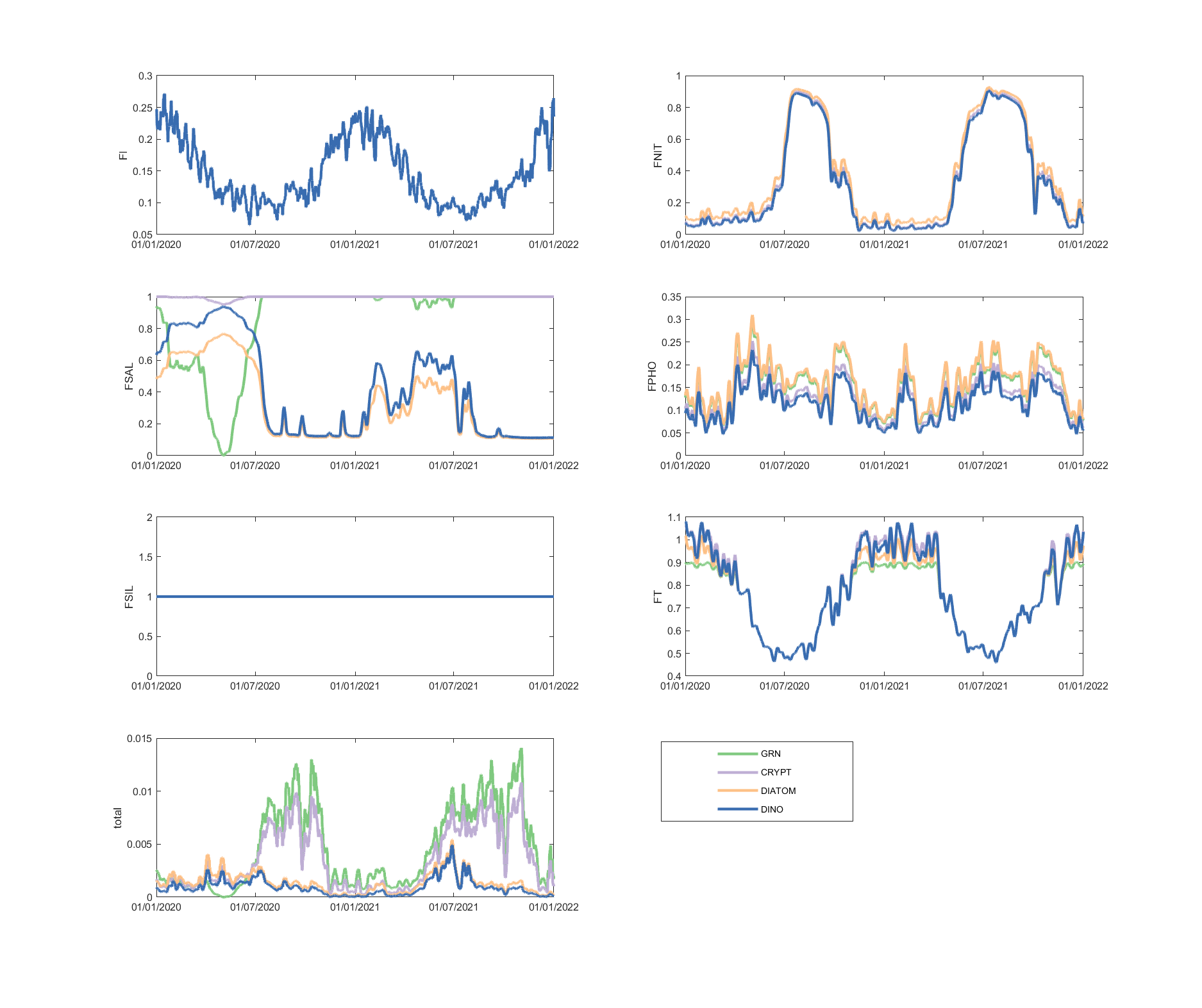
Figure 5.9: Phytoplankton environmental limitation controlling the photosynthesis rate of each phytoplankton group, for site A4261036.

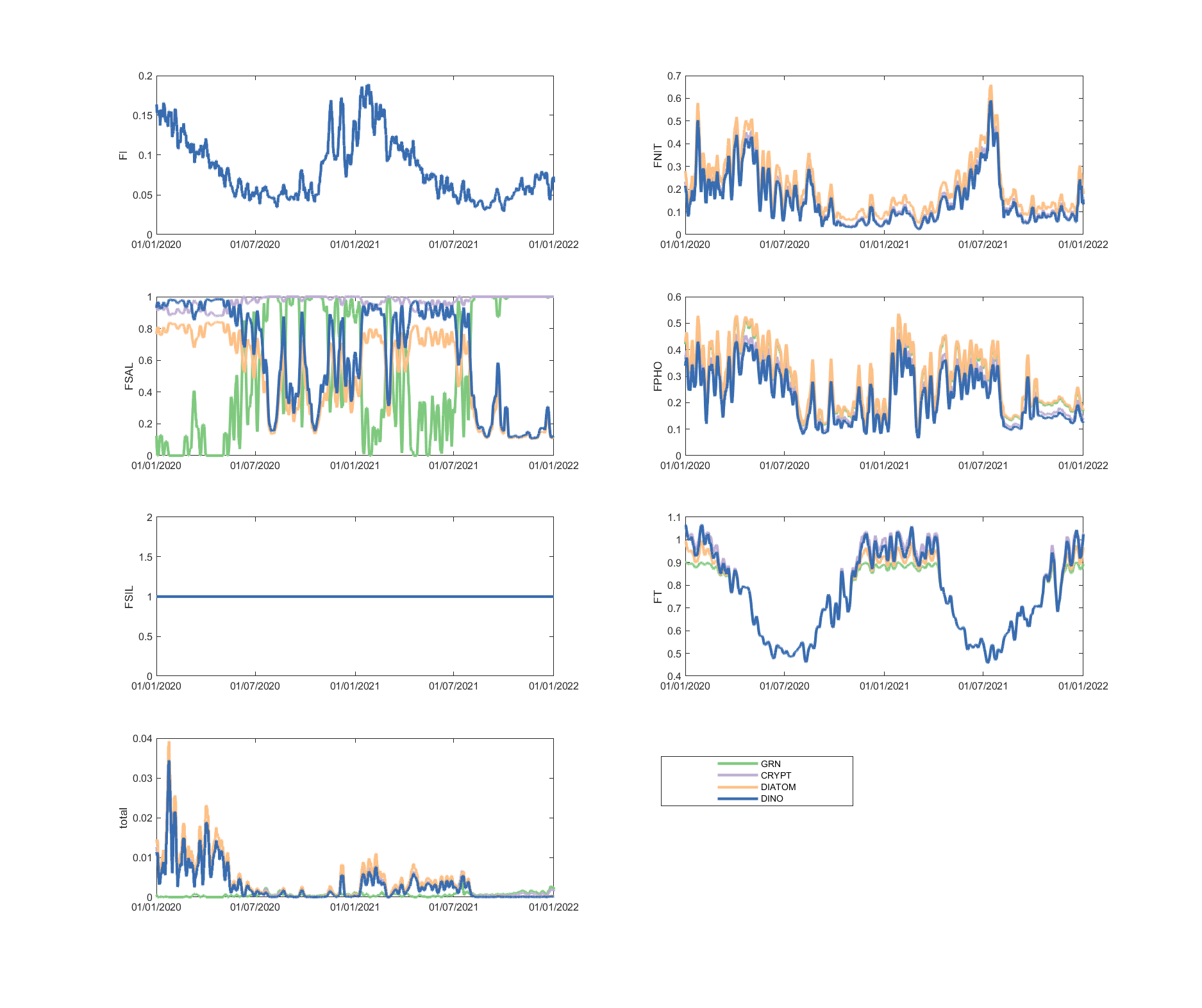
Figure 5.10: Phytoplankton environmental limitation controlling the photosynthesis rate of each phytoplankton group, for site A4261039.

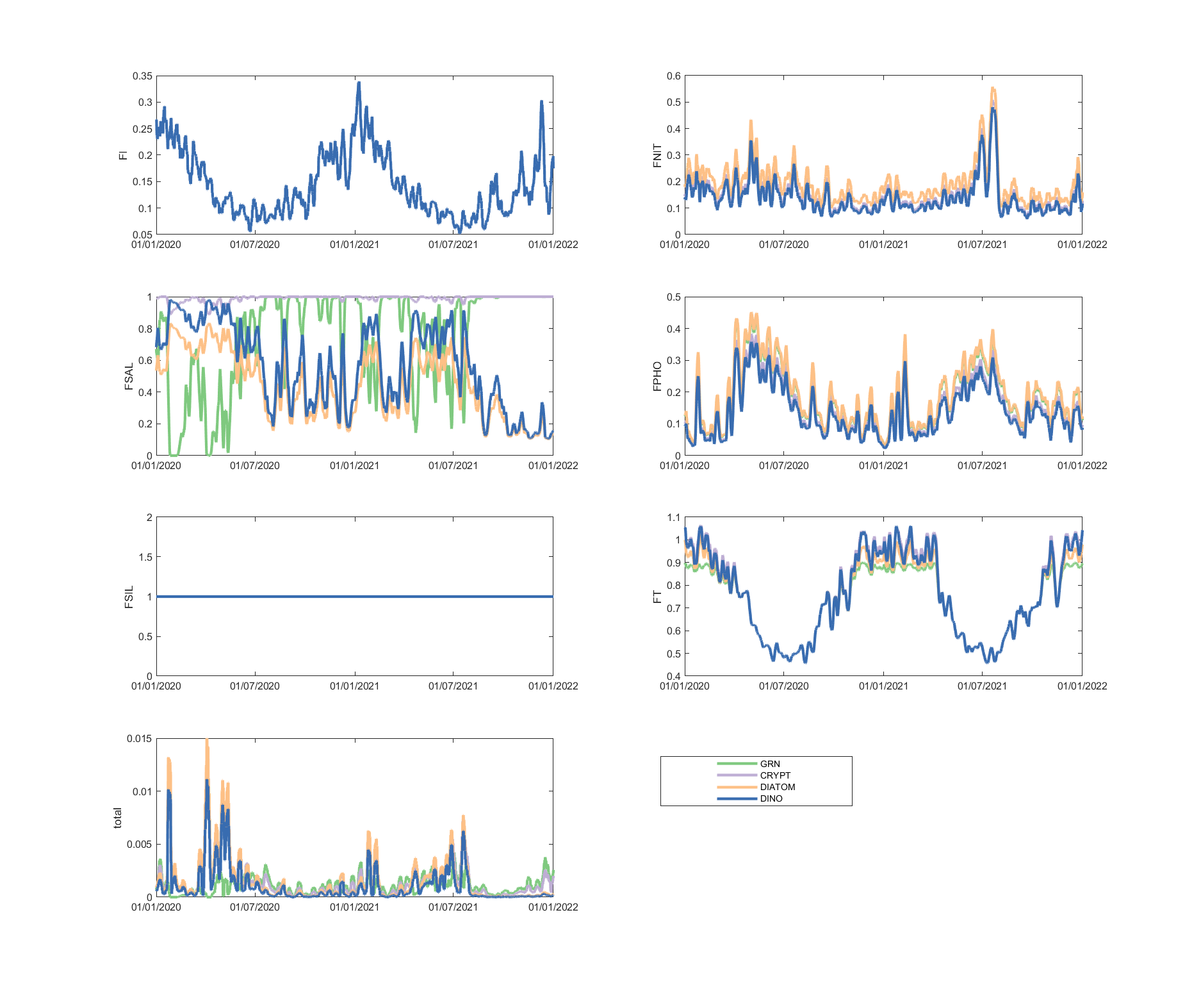
Figure 5.11: Phytoplankton environmental limitation controlling the photosynthesis rate of each phytoplankton group, for site A4261134.

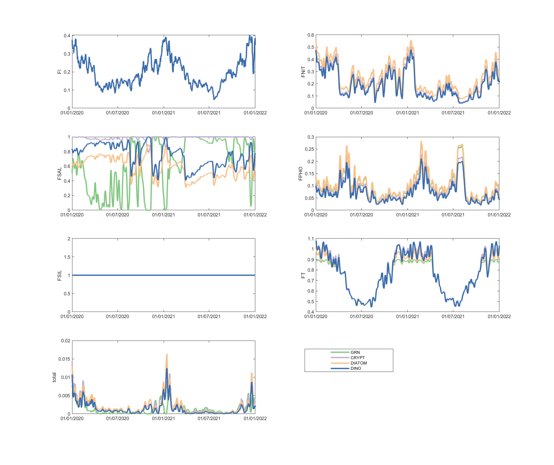
Figure 5.12: Phytoplankton environmental limitation controlling the photosynthesis rate of each phytoplankton group, for site A4261135.

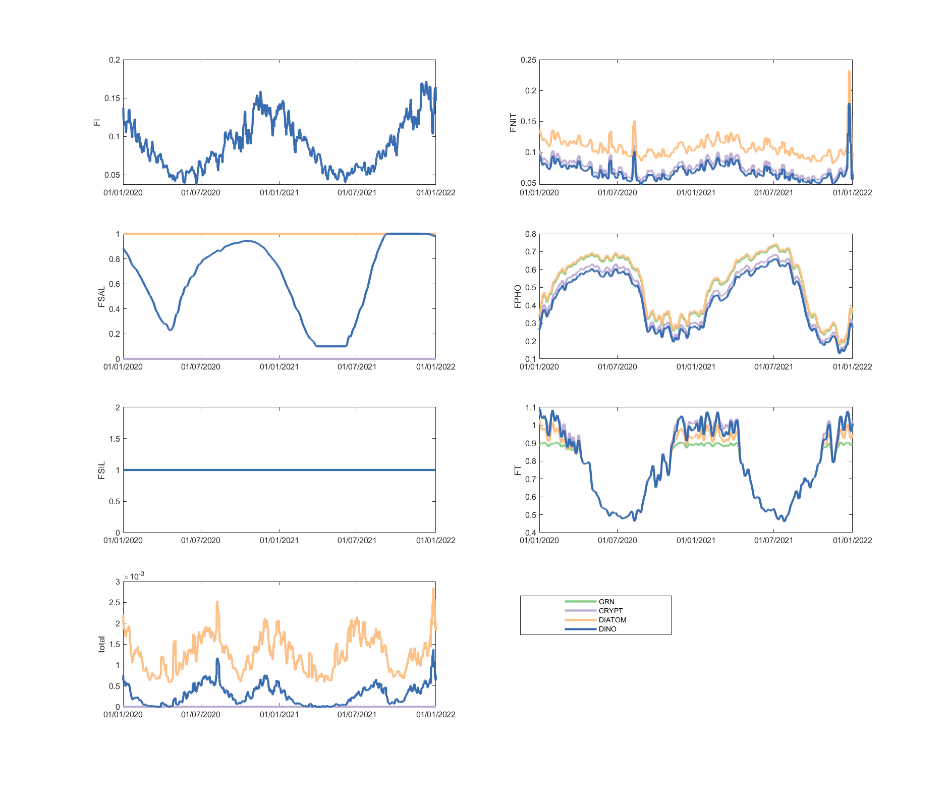
Figure 5.13: Phytoplankton environmental limitation controlling the photosynthesis rate of each phytoplankton group, for site A4261165.

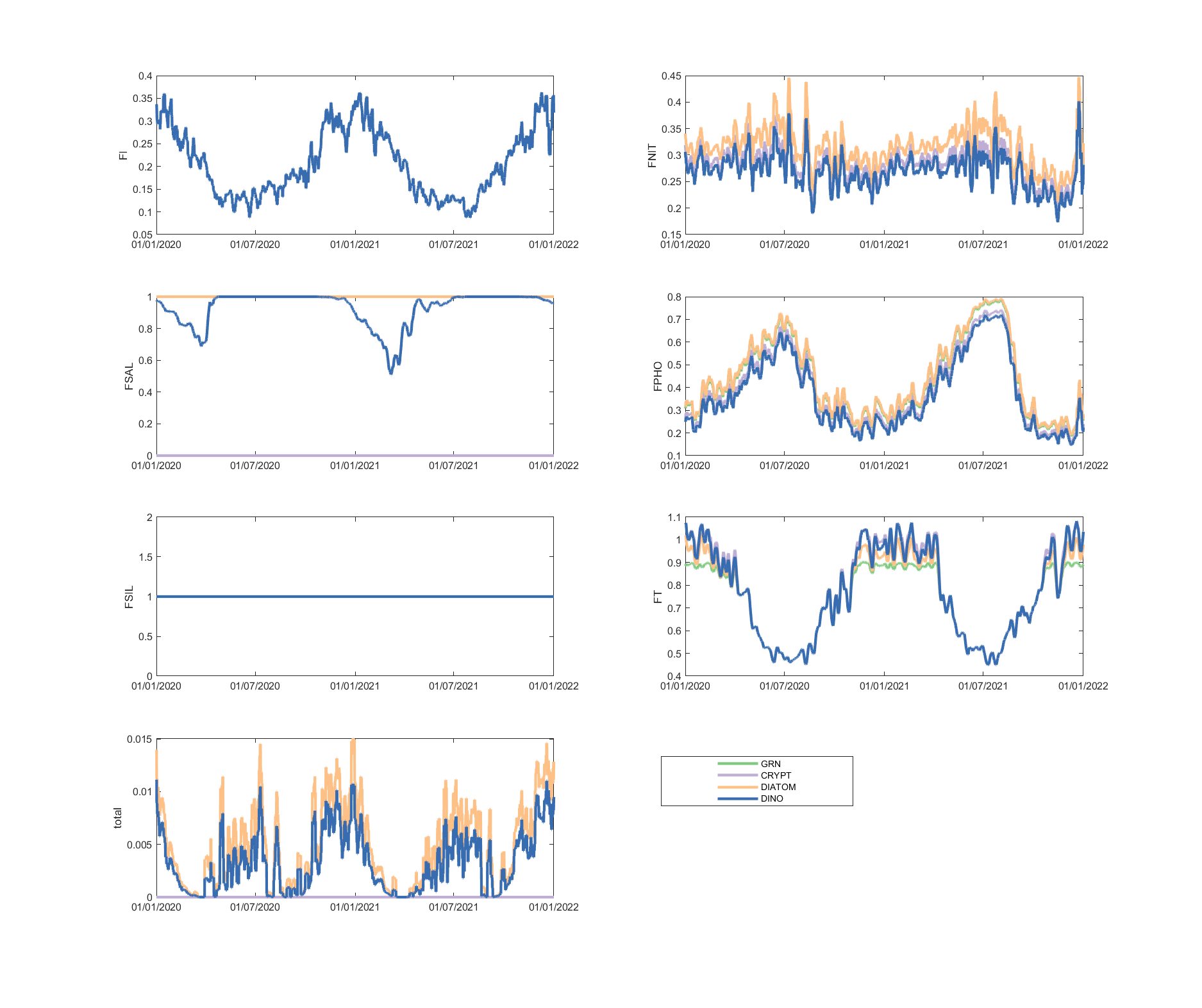
Figure 5.14: Phytoplankton environmental limitation controlling the photosynthesis rate of each phytoplankton group, for site A4261209.

5.5 Summary