9 Integrated Assessment
9.1 Overview
The previous chapters have detailed the nature of the model setup, additions and areas of development. In this section, the model is assessed in its entirety, for each version of the fully coupled model, against the complete dataset. The approach to assess the model aims to follow the CSPS framework of (Hipsey et al., 2020). The framework considers:
- Level 0: conceptual evaluation; the conceptual diagrams for each of the water quality variables, biogeochemical reactions, and habitat modelling are based on the scientific review and data inspection as detailed in the previous chapters;
- Level 1: simulated state variables; a range of metrics is used for a large number of predicted variable and different sites.
- Level 2: process rates; and
- Level 3: system-level patterns and emergent properties; this is evaluated by the overall nutrient budget analysis, nutrient cycling pathway analysis, and assessment of the relationship between the areas of habitat for Ruppia and Ulva.
The specific data available for validation and the assessment metrics used are described next. The level of model uncertainty is discussed in terms of how much confidence is in the current generation of model outputs for the purposes of defining model reliability. As the model is continuously evolving, we report performance based on the model generation.
In addition to the model performance assessment, the model is also routinely used to support management decision-making. Detail is provided on how the diverse model outputs can be processed and analysed for informing the Coorong Decision Making Framework (DMF) and other applications.
9.2 Integrated simulations
A summary of the model lineage and provenance of the different simulations that have been assessed include:
Generation 0 model : Original mesh, 2D hydrodynamics, no surface wave coupling, 1 overall phytoplankton functional group, 5 sediment zones with statically assigned flux rates based on assumed parameters.
Generation 1 model : Original mesh, 2D hydrodynamics, no surface wave coupling, 1 overall phytoplankton functional group, 5 sediment zones with statically assigned flux rates, updated based on observed estimates.
Generation 1.5 model : Original mesh, 2D hydrodynamics, surface wave coupling, 4 phytoplankton functional groups, 31 sediment zones with statically assigned flux rates based on observed parameters.
Generation 2.0 model : Habitat optimised mesh, 2D/3D hydrodynamics, surface wave coupling, 4 phytoplankton functional groups, 31 sediment zones including optional simulation of dynamic, depth-resolved sediment properties, revised life-stage specific macroalgae model, and updated Ruppia habitat thresholds. Uses the 2.0.5 release AED code-base.
Generation 2.1 model : Based on Gen 2.0, refined domain, mesh, bathymetry and material zones to integrate the lastest datasets and improve the Ruppia and macroalgae performance, and update model run time to Nov 2022.
The results from Generation 0 model and Generation 1 model have been reported separately (and their results archived in Appendix B : Results Archive). In this chapter, we focus on the results from the Generation 1.5 and Generation 2 simulations that include the model developments related to the biogeochemistry and habitat, as detailed in the previous chapters. To access a specific model version, refer to the CDM version downloads within GitHub.
9.3 Model assessment approach
9.3.1 Summary of validation data-set
The field observation data available for the model validation and assessment include a diversity of historical data (collected pre 2020), and a large volume of data generated by recent monitoring and HCHB research projects. Relevant data for validation include:
- In situ water quality sensors; high frequency measurements at fixed locations.
- Water quality grab samples
- Biotic surveys
- Strategic experimental data.
All the data relevant to model calibration and validation are included in the CDM Data Catalogue (see Section 3.2) and detailed in Appendix A. The data spans a wide range of locations and time-periods; the most intense period of monitoring is however between 2020-2021 and this serves as the primary model assessment focus period. Long-term assessments are also undertaken for different versions of the model, as outlined next.
9.3.2 Performance assessment metrics
The modelling results are compared against historical data collected within the Coorong (where available), using both traditional statistical metrics of model error, and other metrics relevant to model performance. The approach is applied to each model generation with the aim to identify areas where the model is accurate, and areas for further improvement and ongoing calibration effort.
Error metrics : Initially, the model performance in predicting a range of relevant variables including salinity, temperature, nitrogen, phosphorus and total chlorophyll-a are assessed with a set of statistical metrics, and the calculations of statistical metrics was performed for each observation site where the number of field observations was >10 in the assessment period.
The core statistical metrics considered consist of:
- \(r\): regression coefficient, Varies between -1 and 1, with a score of 1 indicating the model varies perfectly with the observations and a negative score indicating the model varies inversely with the observations. A consistent bias may be present even when high score of r is obtained.
- \(BIAS\): bias of average prediction to the average observation during the assessing period. This method presents a magnitude for the discrepancy between the model results and the observational data.
- \(MAE\): mean absolute error: Similar to RMSE except absolute value is used. This reduces the bias towards large events. Values near zero indicate good model skill.
- \(RMS\): root mean squared error, Measures the mean magnitude, but not direction, of the difference between model data and observations, and hence can be used to measure bias. Values near zero are desirable. This method is not affected by cancellation of negative and positive errors, but squaring the data may cause bias towards large events.
- \(nash\): the Nash-Sutcliffe metric (also called \(NSE\) or \(MEF\) is a matrix of modelling efficiency, measures the mean magnitude of the difference between model data and observations. This method compares the performance of the model to that only uses the mean of the observed data. A value of 1 would indicate a perfect model, while a value of zero indicates performance similar to simply using the mean of observed data.
Seasonality : The model results are assessed in terms of the degree of seasonal fluctuation, as seen in the field data. Whilst this is captured in the error metrics (e.g. R, the visual assessment can assess timing issues related with seasonal peaks.
Transects : The model results are assessed in terms of the seasonal mean along the length of the domain (longitudinal transect). The transect analysis allows a system wide scale assessment of conditions, that smooths out noise and local variability in the field and model predictions.
Advanced measures : The model results were finally assessed considered that partitioning of nutrients in terms of inorganic vs organic, and other expected measures.
Confidence : Based on the above assessment we evaluate confidence in the model by assigning each variable to the following categories:
- Good
- Acceptable, and
- Caution.
This confidence evaluation, considers:
- Quality of observed data, which is influenced by field and laboratory data limitations, methodologies, processes and protocols.
- Error metric scores relative to what is typically reported in the literature for water quality models (e.g., Arhonditsis and Brett (2004) ).
- Ability of the CDM to capture the mean of an indicator and its spatial gradient and seasonality.
- Partitioning of water quality constituents within different ecosystem pools.
- Natural variability of the indicator at different temporal scales (i.e. sub-daily to seasonal).
9.4 Assessment and validation periods
- CIIP period: 2013-2019: initial assessment prior to availability of HCHB research project data;
- Focus period: 2020-2021: initial calibrated against the intensive field sampling and observations obtained from different components of the HCHB research project;
- Long-term performance: 2017 – 2021: calibrated against the long-term water quality data collected from the routine measurements, as well as from the HCHB research project. These results are summarised here.
9.5 Integrated simulation performance
9.5.1 Generation 0
With the Generation 0 model compiled boundary conditions (tide, barrages, Salt Ck inflows) and BARRA weather forcing, the performance of the model in reproducing the long-term nutrient pools has been examined. A summary of model performance is provided in Table 6.1. The full set of time-series validation plots against comparing the model with field observations of salinity, temperature, phytoplankton, and nitrogen/phosphorus species are included in Appendix B1. In summary, the Generation 0 model predicted well the temporal and spatial variations in TN and TP concentrations. However, this version of the model poorly predicted the phytoplankton concentration in the South Lagoon. A reason for this may be due to the fact that this version is run in 2D mode which assumes the water column is fully mixed; whilst the phytoplankton samples were taken in the surface water where the phytoplankton can accumulate.
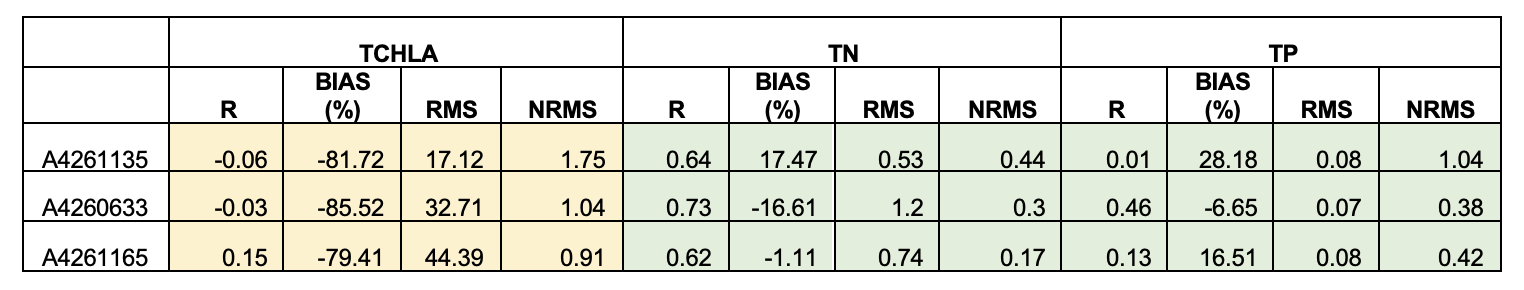
Figure 9.1: Performance summary of CDM (Gen 0) simulating long-term TCHLA, TN and TP concentrations.
The release of bioavailable nutrients is also subject to change once the sediment modelling is completed and the accuracy resolving bioavailable nutrients is still weak. Examination of phytoplankton and nutrient data (see CDM sensitivity assessment to internal loading in appendix B2), and implmentation of 3D dynamics is under development with the Generation I model to capture the vertical distribution of phytoplankton biomass.
9.5.2 Generation 1.5
With the Generation I.5 model compiled boundary conditions (tide, barrage flows, Salt Ck inflows) and weather forcing data from Narrung, the performance of the model in reproducing the long-term nutrient pools has been examined in detail. A brief summary of model performance is provided in Table 6.1. The full set of time-series validation plots against comparing the model with field observations of salinity, temperature, phytoplankton, and nitrogen/phosphorus species are included in Appendix B1. In summary, the Generation I.5 model generally predicted well in most of the variables, including temperature, salinity, TN, TOC, DOC, ammonium and TSS. However, the results in total chlorophyll-a (TCHLA), TP, PO4 and turbidity are relatively poor. On the top of model setting reasons, some reasons for this also come from the data quality, such as:
- The concentration of some of the nutrient species (such as ammonium, nitrate, and phosphate) are lower than the laboratory detective limits, therefore not able to properly evaluate the performance in these species; an example of this is shown in Figure 6.1, which shows the measured nitrate concentration was consistent at 0.003 mg/L (the lowest laboratory detective level for nitrate at UA) from 07/2018 to 01/2020 in zone 42.
- The field observational data were provided from different labs, where the data quality was not consistent; an example of this is shown in Figure 6.2, which shows the TP concentration varied between 0.1-0.4 mg/L before 07/2020, then raised to >5 mg/L after the data source changed to ALS from 07/2020. A similar plot for TN is provided in Figure 6.3, where the TN time series pattern also changed from 07/2020.
Given the fact that the ALS dataset largely departs from the historical data range, a new validation was performed with all existing data except the ALS dataset. A separate summary of model performance is provided in Table 9.2, and the full set of time series validation plots are included in Appendix B. It can be seen from Table @ref(fig:ass-ass15_1) - @ref(fig:ass-ass15_1) that all performance scores of CDM are significantly improved and the performance in most of the water quality prediction are satisfying.
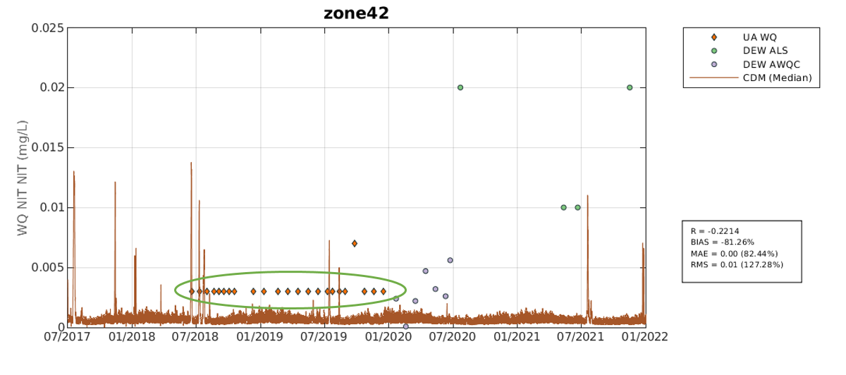
Figure 9.2: Example of data quality issue with modelled vs. measured nitrate concentration in zone 42. Note the consistent nitrate concentration of 0.003 mg/L from 07/2018 to 01/2020 (circled in green).
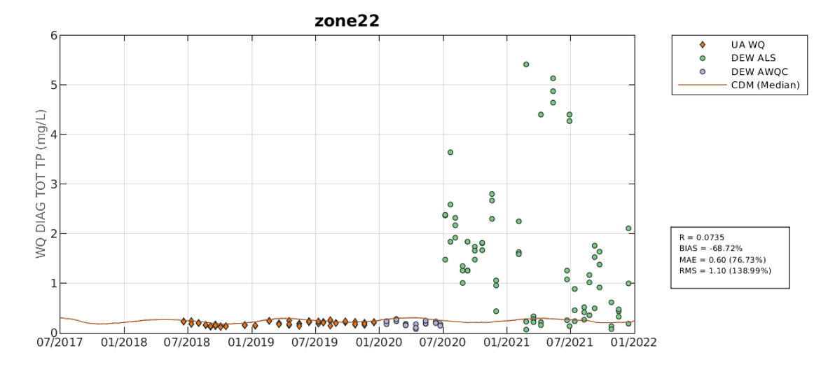
Figure 9.3: Example of data quality issue with modelled vs. measured TP concentration in zone 22. The colours of the observational data indicate their data sources.
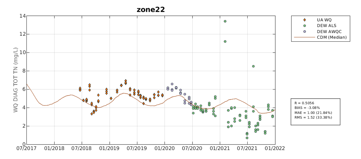
Figure 9.4: Same as Figure 6.2 except for TN concentration in zone 22.
Model performance assessment (no ALS data)
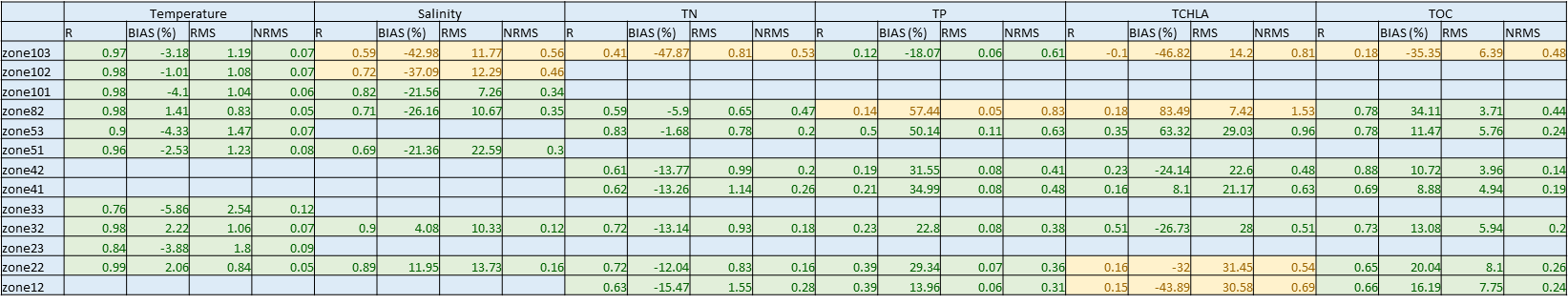
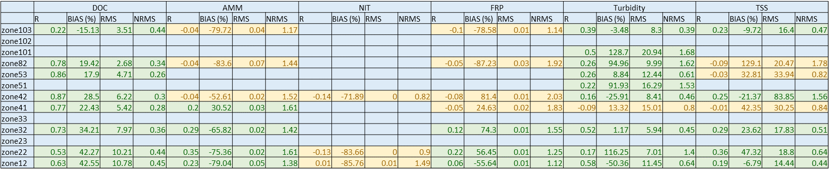
Figure 9.5: Performance summary of CDM (GEN 1.5) simulating long-term temperature, salinity, and nutrient concentrations, validated with all existing data available (inlcuding ALS). Red indicates a poor calibration result suggesting those variables should be considered with caution, yellow indicates an acceptable level of performance, and green indicates anaccurate prediction. Click to enlarge.
Model performance assessment (all data)
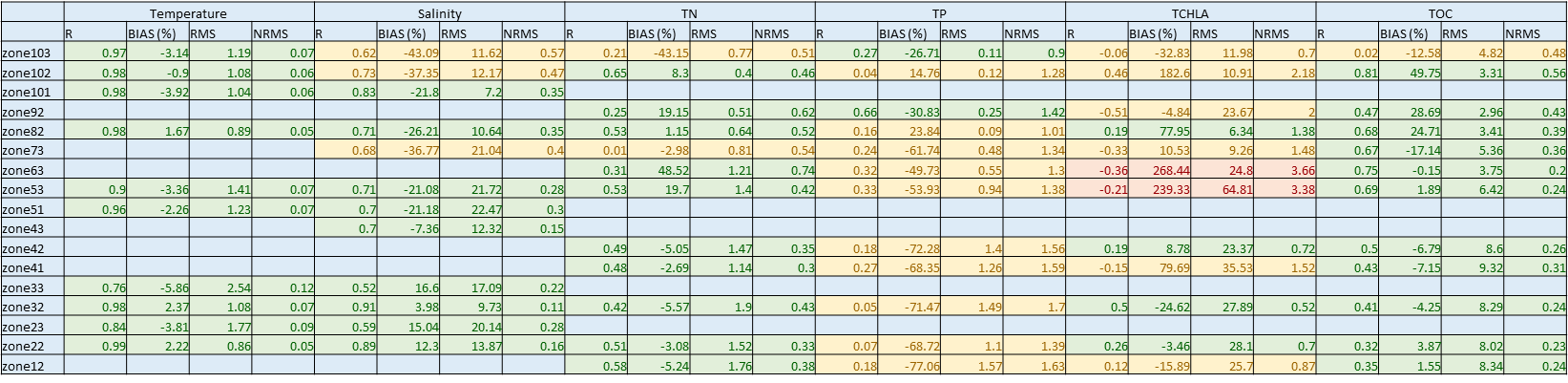
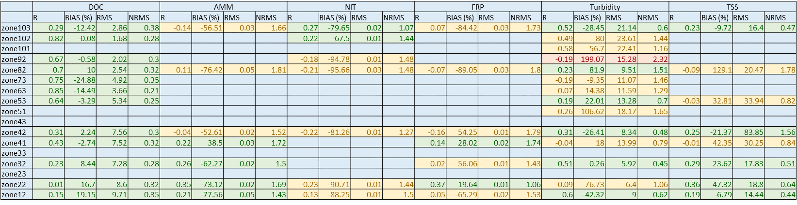
Figure 9.6: Performance summary of CDM (GEN 1.5) simulating long-term temperature, salinity, and nutrient concentrations, validated with all existing data except the laboratory data from ALS. Red indicates a poor calibration result where results should be considered with caution, yellow indicates an acceptable level of performance, and green indicates a highly accurate prediction. Click to enlarge.
9.5.3 Generation 2.0
The error metrics for the Generation 2.0 simulation are shown below.
Model performance assessment (no ALS data)
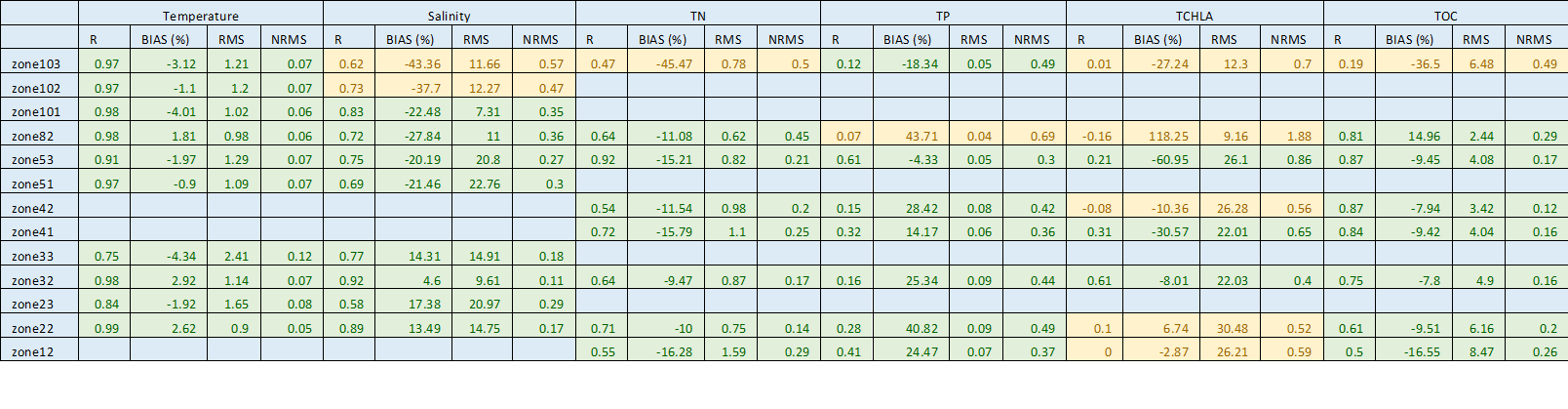
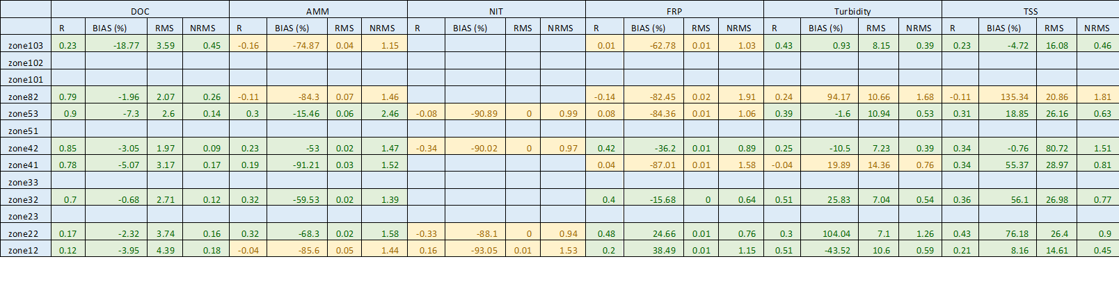
Figure 9.7: Performance summary of CDM (GEN 2.0) simulating long-term temperature, salinity, and nutrient concentrations, validated with all existing data available (inlcuding ALS). Red indicates a poor calibration result suggesting those variables should be considered with caution, yellow indicates an acceptable level of performance, and green indicates anaccurate prediction. Click to enlarge.
Model performance assessment (all data)
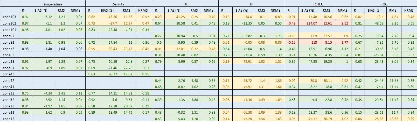
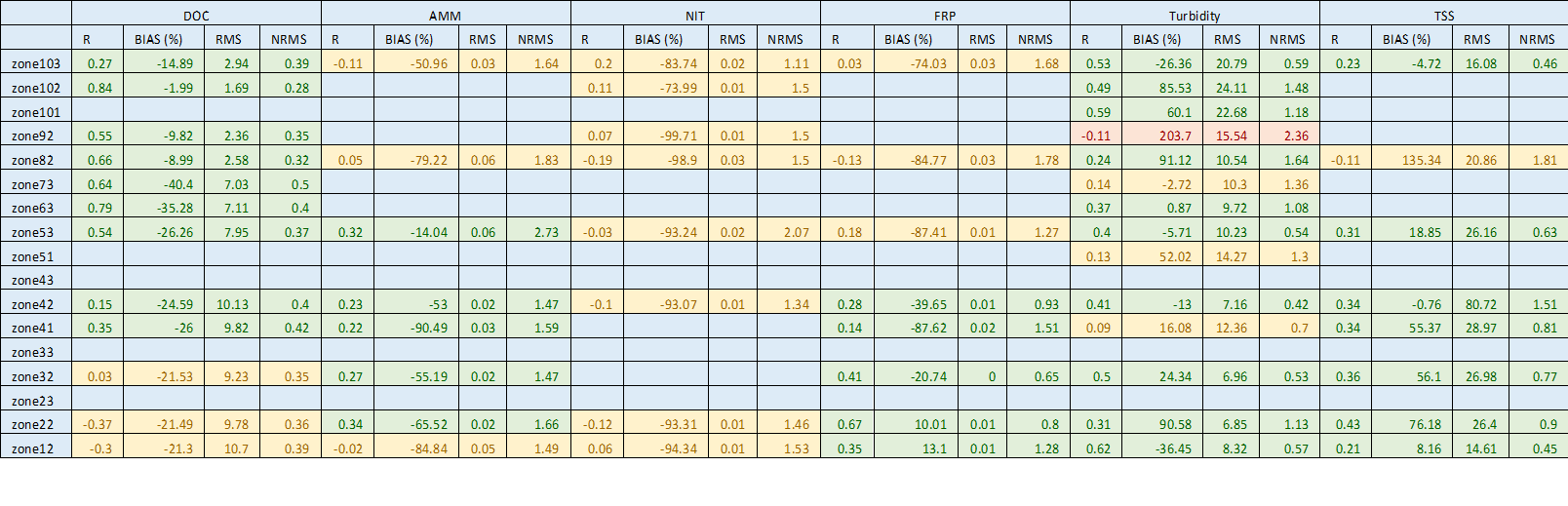
Figure 9.8: Performance summary of CDM (GEN 2.0) simulating long-term temperature, salinity, and nutrient concentrations, validated with all existing data except the laboratory data from ALS. Red indicates a poor calibration result where results should be considered with caution, yellow indicates an acceptable level of performance, and green indicates a highly accurate prediction. Click to enlarge.
9.5.4 Generation 2.1
The error metrics for the Generation 2.1 simulation are shown below.
Model performance assessment (no ALS data)
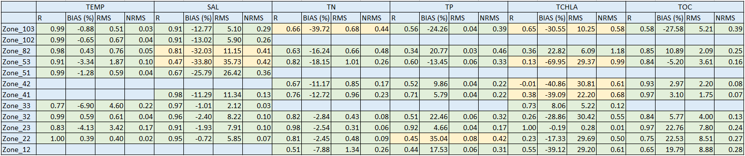
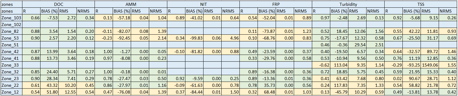
Figure 9.9: Performance summary of CDM (GEN 2.1) simulating long-term temperature, salinity, and nutrient concentrations, validated with all existing data available (inlcuding ALS). Red indicates a poor calibration result suggesting those variables should be considered with caution, yellow indicates an acceptable level of performance, and green indicates anaccurate prediction. Click to enlarge.
9.6 Nutrient budget assessment
9.6.1 Nutrient budgets
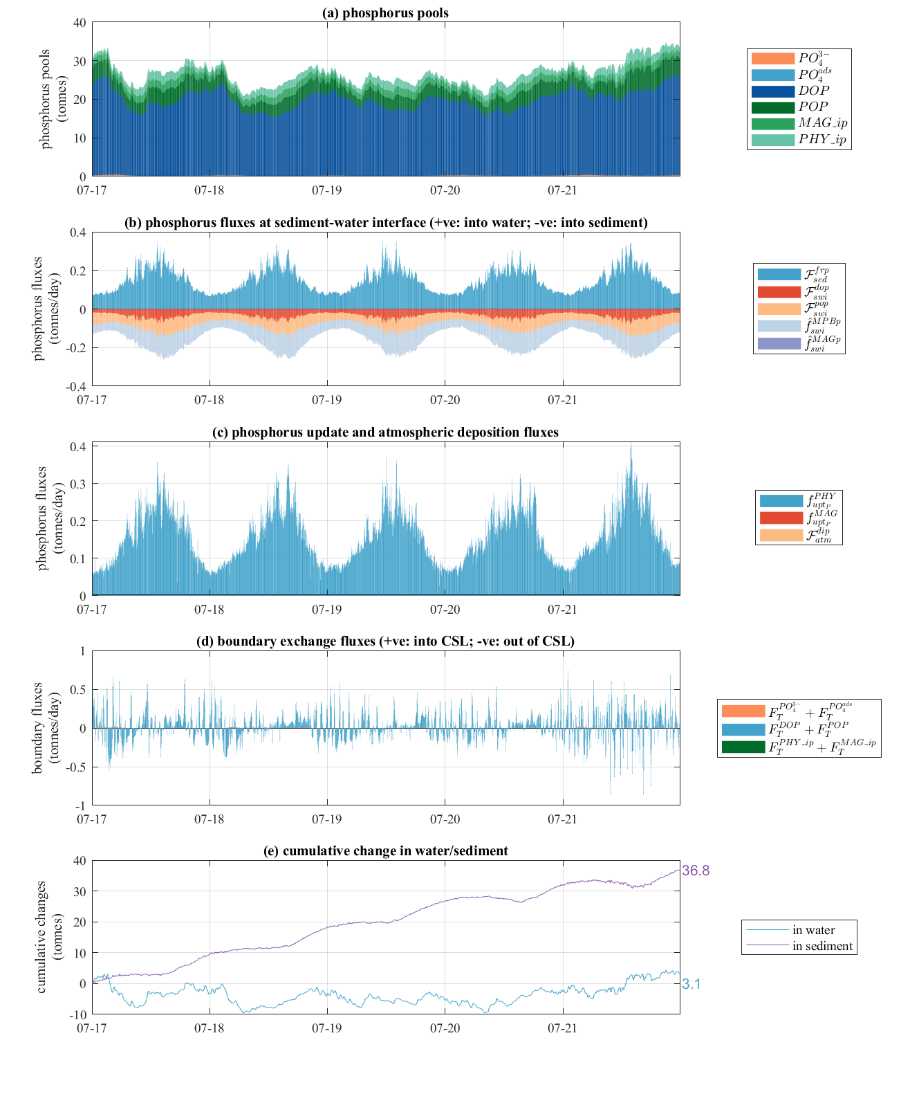
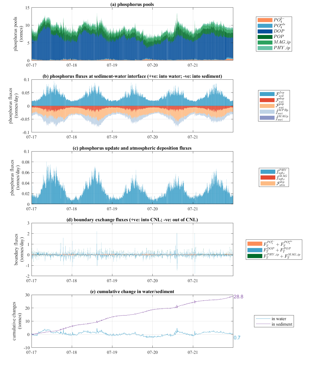
A methodology for nutrient flux and budget analysis has been developed. For the nutrient budget analysis, all of the nutrient pools (dissolved and particulate carbon, nitrogen and phosphorus, macroalgae and Ruppia) can be summarized for different regions of the estuary (north, south etc.). As an example of this method, the results from a period of five years (01/07/2017 to 01/07/2022) were summarized for nitrogen budgeting of NCL and SCL region in Figure 9.9 - 9.12. The nutrient budgeting analysis showed that the dissolved organic matter is the major nitrogen pool in both the lagoons, while particle organic matter and the nitrogen assimilated by phytoplankton also presented to be major nutrient pools (panel “a”). The sediment diffusion release of ammonium and the nitrogen loss due to phytoplankton burial into the sediment dominate the interaction at the sediment-water interface (panel “b”), which also presented a clear seasonal pattern. The boundary exchange fluxes are dominated by the organic matters in coincident to the major pools in the water (panel “c”). The daily change flux rate varied between 0 to >20 tonne/day in the north lagoon, compared to that of between 0 to ~10 tonnes/day in the south lagoon, indicating stronger hydrodynamic transportation in the north lagoon affected by tidal intrusion and barrage flow. The results showed a net cumulative of nutrient in the sediment (panel “d”), indicating the sediment acting as a sink for the nutrients.
NITROGEN (CSL)
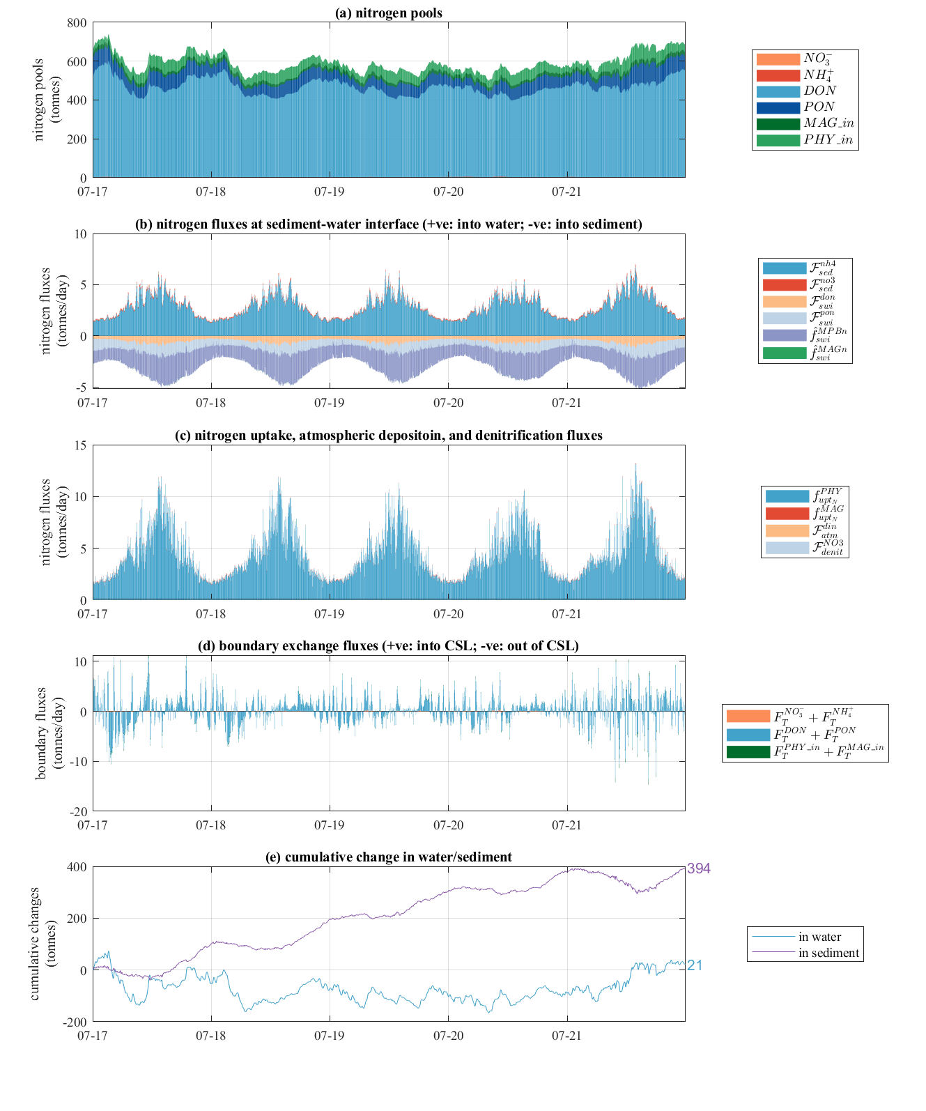
Figure 9.10: Time-series plot of daily changes in (a) nitrogen pools, (b) nitrogen sources and sinks at the atmospheric and sediment interfaces, (c) exchange fluxes at the boundaries, and (d) cumulative changes in water and sediment of the south lagoon.
NITROGEN (CNL)
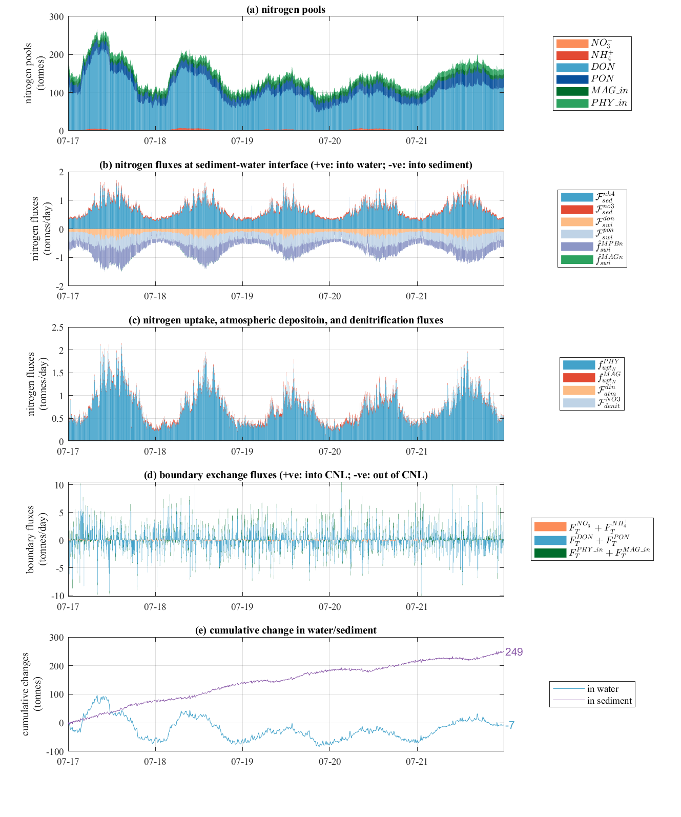
Figure 9.11: Time-series plot of daily changes in (a) nitrogen pools, (b) nitrogen sources and sinks at the atmospheric and sediment interfaces, (c) exchange fluxes at the boundaries, and (d) cumulative changes in water and sediment of the north lagoon.
9.6.2 Source and sink summary
Averaging the nitrogen and phosphorus pathways over the 5-year study period highlights the general fate of external nutrient loads entering the system, which is conceptualised as the Coorong “conveyer belt” (Figure 9.13). In summary, the nutrient loads with the barrage flows were the dominant source, representing 99% of total catchment nutrient load from the barrages and Salt Creek. There was active exchange of water and nutrient at the Murray mouth, where most of the nitrogen and phosphorus entering the Coorong through the barrages were exported to the ocean. The net fluxes transported to the CNL and to the CSL showed a gradual decrease, indicating decreasing connectivity from north to south. In CNL, the nitrogen fluxes by sediment release and settling were in the same order to that by transport into the CNL. While in CSL, the internal sediment fluxes were one order higher to that by transport through the boundary. However, although there was fast exchange of nitrogen at the sediment-water interface, the net accumulation in the CSL sediment of nitrogen (4.0% of total catchment load) and of phosphorus (4.1% of total catchment load) was relatively slow and in same order to the boundary exchange.
Figure 9.14: Summary pie chart of nitrogen sources and sinks in the north lagoon (NCL) and south lagoon (SCL).
9.7 Environmental response function (ERF) analysis
A useful method for applying the model is to construct environmental response function (ERFs); these can be used to predict water quality variables in estuary/lagoon sub-domains in response to changes in boundary forcing, and can therefore provide a simple and quick assessment of the occurrence of some target events. As an example, the environmental response of salinity, TN and TP in space and time is compared for a scenario assessing the delivery of water for the environment. This compares how the lagoon differs in repsonse to water being provided as an “environmental flow” (e.g. see Brookes et al. (2022) ). Two simulations are compared:
- ‘all water’ : representing the base-case scenario where water was delivered over the barrages as actually occurred, and
- ‘no-eWater’ : representing a counter-factual situation when there was no environmental water delivered across the barrages
The results demonstrate that, under the current condition, the annual-average salinity presented an increase from north the south, and the condition stayed similar from 2017 to 2021; while if there is no environmental water contribution (the ‘no-eWater’ scenario), the salinity would had increased from about 150 PSU in 2017 to near 190 PSU in 2021 (Figure 9.15). The nutrient levels showed an increase from north to south, and also increased with time in both scenarios. However, if there is no environmental water contribution, the TN and TP in the south lagoon would have increased at a faster pace. In summary, the environmental water has shown to help to reduce the salinity level as well as the trophic statues of the Coorong, and show how the model can be used to develop ‘look-up’ tables for expected benefits of a given change in operation, without running the full model.
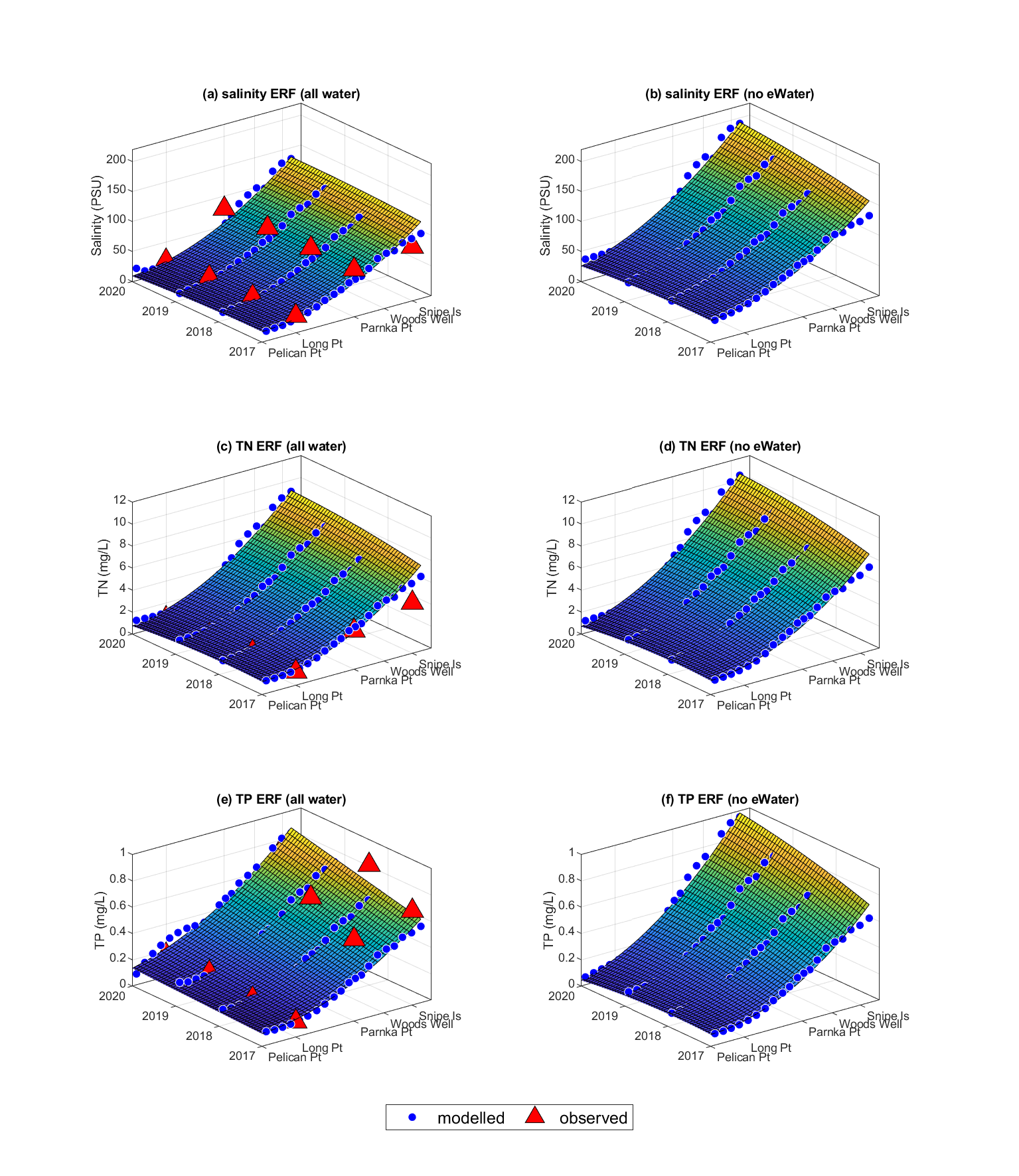
Figure 9.15: Environmental response functions (ERF) of salinity, TN, and TP in space and time of the Coorong for the base-case scenario (left panel) and an example ‘no e-Water’ scenario (right panel).
9.8 Habitat condition assessment
The overall habitat suitability for sexual and asexual reproduction between 2018 - 2021 have been simulated using the Gen 2 model (Figure 9.16 and Figure 9.17). The results show that habitat quality and suitable area can shift from year to year. For exmaple, in comparison, 2021 offered the least amount of suitable habitat for Ruppia to complete its sexual life cycle (flowering), which was consistent with field observations in that very few flowers were recorded in 2021 compared to 2020.
Ruppia HSI (sexual lifecycle)
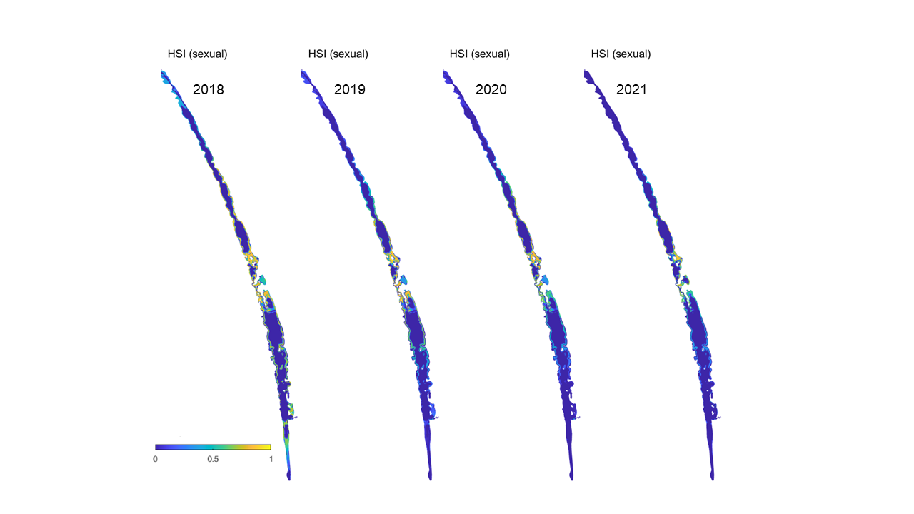
Figure 9.16: Overall Habitat Suitability Index for the successful completion of the sexual life cycle in the Coorong, for the Base Case in 2018 - 2021. An HSI of 0 (dark purple) represents unsuitable habitat conditions, while an HSI of 1 represents optimal conditions (yellow).
Ruppia HSI (asexual lifecycle)
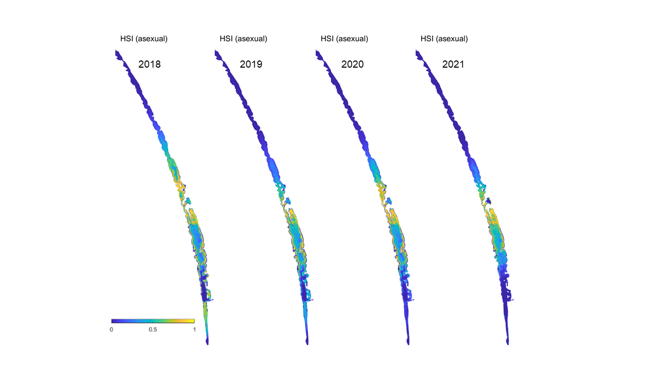
Figure 9.17: Overall Habitat Suitability Index for the successful completion of the asexual life cycle in the Coorong, for the Base Case in 2018 - 2021. An HSI of 0 (dark purple) represents unsuitable habitat conditions, while an HSI of 1 represents optimal conditions (yellow).
9.9 Coorong Decision Making Framework (DMF)
To facilitate management decision making, and comprehensive list of customised model post-processing exports has been created. The Decision Making Framework (DMF) exports encompass a wide range of critical “CPS” indicators. These are defined in Table 9.1.
| Indicator | Time | Space | Measure |
|---|---|---|---|
| Ruppia | |||
| Life stage: turion viability | Jan-Mar | CNL | HSI × Area |
| Life stage: turion viability | Jan-Mar | CSL | HSI × Area |
| Life stage: seed germination | Apr-July | CNL | HSI × Area |
| Life stage: seed germination | Apr-July | CSL | HSI × Area |
| Life stage: Turion sprouting | Apr-July | CNL | HSI × Area |
| Life stage: Turion sprouting | Apr-July | CSL | HSI × Area |
| Life stage: Adult plant growth | June-Sept | CNL | HSI × Area |
| Life stage: Adult plant growth | June-Sept | CSL | HSI × Area |
| Life stage: Flowering | Aug-Dec | CNL | HSI × Area |
| Life stage: Flowering | Aug-Dec | CSL | HSI × Area |
| Life stage: Turion production | Aug-Dec | CNL | HSI × Area |
| Life stage: Turion production | Aug-Dec | CSL | HSI × Area |
| Life stage: Seedbank production | Aug-Dec | CNL | HSI × Area |
| Life stage: Seedbank production | Aug-Dec | CSL | HSI × Area |
| Lifecycle | June-Dec | CSL | HSI × Area |
| Lifecycle | June-Dec | CNL | HSI × Area |
| Oxygen penetration depth (sediment) | Apr-July | CNL & CSL | Average daily area (Km2) where OPD is =3 cm using shallow sediment zones |
| Oxygen penetration depth (sediment) | June-Sept | CNL & CSL | Average daily area (Km2) where OPD is =3 cm using shallow sediment zones |
| Oxygen penetration depth (sediment) | Aug-Dec | CNL & CSL | Average daily area (Km2) where OPD is =3 cm using shallow sediment zones |
| Macroinvertebrates | |||
| Water depth and salinity | Apr-Sep | System-wide | Average daily area (Km2) with water cover and <25 g/L |
| Water depth and salinity | Oct-Mar | System-wide | Average daily area (Km2) with water cover and <25 g/L |
| Water depth and salinity | Apr-Sep | System-wide | Average daily area (Km2) with water cover and <50 g/L |
| Water depth and salinity | Oct-Mar | System-wide | Average daily area (Km2) with water cover and <50 g/L |
| Water depth and salinity | Apr-Sep | System-wide | Average daily area (Km2) with water cover and <105 g/L |
| Water depth and salinity | Oct-Mar | System-wide | Average daily area (Km2) with water cover and <105 g/L |
| Macroalgae | Apr-Sep | System-wide | Area (Km2) of Algae HSI >0.25 |
| Macroalgae | Oct-Mar | System-wide | Area (Km2) of Algae HSI >0.25 |
| Oxygen penetration depth (sediment) | Apr-Sep | System-wide | Average daily area (Km2) where OPD is =3 cm using shallow sediment zones |
| Oxygen penetration depth (sediment) | Oct-Mar | System-wide | Average daily area (Km2) where OPD is =3 cm using shallow sediment zones |
| Fish diversity (species richness/biodisparity | |||
| Salinity | Apr-Sep | ME | Mean daily longitudinal extent (km) below 30 g/L |
| Salinity | Oct-Mar | ME | Mean daily longitudinal extent (km) below 30 g/L |
| Salinity | Apr-Sep | System-wide | Mean daily longitudinal extent (km) below 60 g/L |
| Salinity | Oct-Mar | System-wide | Mean daily longitudinal extent (km) below 60 g/L |
| Salinity | Year-round | ME | No. of events that mean monthly estuary-averaged salinity (via stations A4261036, A4261039, A4261128, A4261043) is >40 g/L for =2 months |
| Flow (River Murray discharge) | Year-round | Boundary condition | Average monthly River Murray (barrages) discharge (GL) |
| Murray Mouth morphology | Year-round | ME | % of days where Murray Mouth depth is = 1 m |
| Smallmouth hardyhead (Foodweb) | |||
| Salinity | Apr-Sep | System-wide | Mean daily longitudinal extent (km) below 100 g/L |
| Salinity | Oct-Mar | System-wide | Mean daily longitudinal extent (km) below 100 g/L |
| Flow (River Murray discharge) | Sep-Mar | Boundary condition | Average monthly River Murray discharge (GL) |
| Water level | Apr-Sep | CSL | % of days when CSL average water level is >0.3 m AHD |
| Water level | Oct-Mar | CSL | % of days when CSL average water level is >0.3 m AHD |
| South East connectivity (fishway operation) | Apr-Sep | CSL | % of days where Salt Creek flow is >3 ML/day and average CSL is >+0.4 m AHD or Salt Creek flow is >2 ML/day and average CSL is >+0.8 m AHD |
| South East connectivity (fishway operation) | Oct-Mar | CSL | % of days where Salt Creek flow is >3 ML/day and average CSL is >+0.4 m AHD or Salt Creek flow is >2 ML/day and average CSL is >+0.8 m AHD |
| Fish movement and recruitment (congolli and common galaxias) | |||
| Flow (River Murray discharge) | May–Aug | Boundary condition | Average monthly River Murray discharge (GL). |
| Flow (River Murray discharge) | Oct–Jan | Boundary condition | % of days when barrage flow are = 200 ML/day. |
| Murray Mouth morphology | May–Jan | ME | % of days where Murray Mouth depth is = 30 cm |
| Salinity | Oct–Jan | ME | % of days where average daily Murray estuary salinity is <35 g/L |
| Waterbirds (Shorebirds) | |||
| Water depth | Sept-Apr | System-wide | Mean average daily Ha of water cover from <10 cm |
| Water depth | Sept-Apr | System-wide | Mean average daily Ha of water cover from <20 cm |
| Water level | Sept-Apr | CSL | % of days that CSL lagoon-averaged water levels are >+0.4 m AHD |
| Salinity | Sept–Apr | System-wide | Mean daily longitudinal extent (km) below 140 g/L |
| Macroalgae | Sept–Apr | System-wide | Mean average daily Ha of algae HSI >0.25 |
| Waterbirds (Waterfowl) | |||
| Ruppia (adult growth) | Apr–Sept (model period with precursor stages) | CNL | HSI × Area |
| Ruppia (adult growth) | Apr–Sept (model period with precursor stages) | CSL | HSI × Area |
| Ruppia (turion) - asexual lifecyle | Turion production: June-Dec (model period with precursor stages) | CNL | HSI × Area |
| Ruppia (turion) - asexual lifecyle | Turion production: June-Dec (model period with precursor stages) | CSL | HSI × Area |
| Water level | Sept-May | CSL | % of days when the lagoon-averaged water level in the CSL is above +0.35 m AHD |
| Waterbirds (Piscivores) | |||
| Salinity | Sept-Apr | System-wide | Mean daily longitudinal extent (km) below 45 g/L |
| Salinity | Sept-Apr | System-wide | Mean daily longitudinal extent (km) below 100 g/L |
| Flow (River Murray discharge) | Sept-Apr | System-wide | Average monthly River Murray discharge (GL) |
| Water level | Sept-Apr | CSL | % of days when the lagoon-averaged water level in the CSL is below -0.5 m AHD |
| Surface water regime | |||
| Flow (River Murray barrages) | Year-round | System-wide | Total barrage release volume (GL) |
| Flow (River Murray barrages) | Year-round | System-wide | <U+0394> from 650 GL/year |
| Flow (River Murray barrages) | Year-round | System-wide | <U+0394> from 2000 GL/year rolling annual average |
| Flow (River Murray barrages) | Year-round | System-wide | <U+0394> from 6,000 GL/year |
| Flow (River Murray barrages) | Year-round | System-wide | <U+0394> from 10,000 GL/year |
| Flow (Salt Creek) | Year-round | CSL | Total flow from Salt Creek (GL) |
| Water level | June-Aug | CSL | % of days CSL lagoon-averaged mean-daily water levels (via CSL stations A4260633, A4261209 and A4261165) are =+0.3 m AHD |
| Water level | June-Aug | CSL | Maximum duration (days) of CSL lagoon-averaged mean-daily water levels (via CSL stations A4260633, A4261209 and A4261165) are <+0.3 m AHD |
| Water level | June-Aug | CSL | % of CSL lagoon-averaged mean-daily water levels (via CSL stations A4260633, A4261209 and A4261165) are <+0.2 m AHD |
| Water level | Sep-Dec | CSL | % of days CSL lagoon-averaged mean-daily water levels (via CSL stations A4260633, A4261209 and A4261165) are =+0.2 m AHD |
| Water level | Sep-Dec | CSL | % CSL lagoon-averaged mean-daily water levels (via CSL stations A4260633, A4261209 and A4261165) are <+0.15 m AHD |
| Salinity | Year-round | ME | % of months that the mean monthly estuary-averaged salinity (via stations A4261036 A4261039, A4261128, A4261043) is <35 g/L |
| Salinity | Year-round | CNL | % of months that the mean monthly lagoon-averaged salinity (via A4261134, A4261135 and A4260572) is <45 g/L |
| Salinity | June-Aug | CSL | % of months that the mean monthly lagoon-averaged salinity (via A4261134, A4261135 and A4260572) is <60 g/L |
| Salinity | Year-round | System-wide | Mean daily longitudinal extent of the Coorong (Km) below 60 g/L |
| Salinity | Year-round | CSL | % of days that the mean daily Lagoon average salinity (via A4261134, A4261135 and A4260572) is <100 g/L |
| Salinity | Year-round | CSL | % of months that the mean monthly lagoon-averaged salinity (via A4261134, A4261135 and A4260572) is >100 g/L |
| Trophic status (threat: eutrophication) | |||
| Total Nitrogen | Apr-Sep | CNL - require spatial dividing line prior to model run - nodestring set-up for model run. | Balance (import – export) (g/kg) at 30 September (or simulation end date) from 1 April (or simulation start date). |
| Total Nitrogen | Apr-Sep | CSL | Balance (import – export) (g/kg) at 30 September (or simulation end date) from 1 April (or simulation start date). |
| Total Nitrogen | Oct-Mar | CNL | Balance (import – export) (g/kg) at 31 March (or simulation end date) from 1 October (or simulation start date). |
| Total Nitrogen | Oct-Mar | CSL | Balance (import – export) (g/kg) at 31 March (or simulation end date) from 1 October (or simulation start date). |
| Total Phosphorus | Apr-Sep | CNL | Balance (import – export) (g/kg) at 30 September (or simulation end date) from 1 April (or simulation start date). |
| Total Phosphorus | Apr-Sep | CSL | Balance (import – export) (g/kg) at 30 September (or simulation end date) from 1 April (or simulation start date). |
| Total Phosphorus | Oct-Mar | CNL | Balance (import – export) (g/kg) at 31 March (or simulation end date) from 1 October (or simulation start date). |
| Total Phosphorus | Oct-Mar | CSL | Balance (import – export) (g/kg) at 31 March (or simulation end date) from 1 October (or simulation start date). |
| Total Chlorophyll-a | Apr-Sep | CNL | Average daily <U+2206> from the mean daily lagoon-averaged T Chl-a concentration |
| T Chl-a | Oct-Mar | CNL | Average daily <U+2206> from the mean daily lagoon-averaged T Chl-a concentration |
| T Chl-a | Oct-Mar | CSL | Average daily <U+2206> from the mean daily lagoon-averaged T Chl-a concentration |
| T Chl-a | Apr-Sep | CSL | Average daily <U+2206> from the mean daily lagoon-averaged T Chl-a concentration |
| Dissolved oxygen | Apr-Sep | ME, CNL | Average daily area (HA) that minimum DO is =6.5 mg/L |
| Dissolved oxygen | Oct-Mar | ME, CNL | Average daily area (HA) that minimum DO is =6.5 mg/L |
| Dissolved oxygen | Apr-Sep | CSL | Average daily area (HA) that minimum DO is =4 mg/L |
| Dissolved oxygen | Oct-Mar | CSL | Average daily area (HA) that minimum DO is =4 mg/L |
| Oxygen penetration depth | Apr-Sep | ME, CNL | Average daily area (Km2) where OPD is =3 cm using shallow sediment zones |
| Oxygen penetration depth | Apr-Sep | CSL | Average daily area (Km2) where OPD is =3 cm using shallow sediment zones |
| Oxygen penetration depth | Oct-Mar | ME, CNL | Average daily area (Km2) where OPD is =3 cm using shallow sediment zones |
| Oxygen penetration depth | Oct-Mar | CSL | Average daily area (Km2) where OPD is =3 cm using shallow sediment zones |
Outputs are initially grouped based upon the style of calculation required.
An example of the outputs can be found in Table 9.2.
| Indicator | Start Time | End Time | Var | Trigger | Area (km2) | Total Area (km2) |
|---|---|---|---|---|---|---|
| Macroinvertebrates | ||||||
| Water depth and salinity | 2020-04-01 | 2020-10-01 | SAL | 25 | 39.4596 | 213.5229 |
| Water depth and salinity | 2020-10-01 | 2021-04-01 | SAL | 25 | 54.3544 | 213.5229 |
| Water depth and salinity | 2020-04-01 | 2020-10-01 | SAL | 50 | 106.7920 | 213.5229 |
| Water depth and salinity | 2020-10-01 | 2021-04-01 | SAL | 50 | 85.0856 | 213.5229 |
| Water depth and salinity | 2020-04-01 | 2020-10-01 | SAL | 105 | 186.3159 | 213.5229 |
| Water depth and salinity | 2020-10-01 | 2021-04-01 | SAL | 105 | 169.1278 | 213.5229 |
In addition to the required DMF value, time series plots are also produced to provide context to the data analyst.
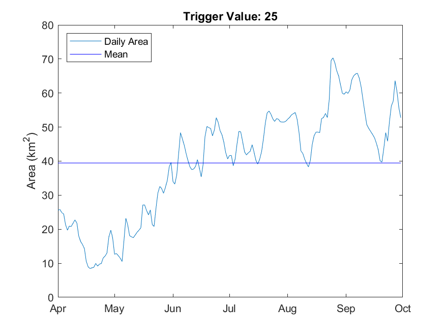
Figure 9.18: Critial CPS for macroinvertabrates where Average daily area (Km2) with water cover and Salinity is < 25 g/L Apr-Sep
9.10 Summary
A series of integrated CDM assessment toolbox has been developed that are able to:
- Accomodate data from different sources/campaigns (see Appendix A)
- Flexible plotting of time-series outputs at points and integrated over polygons
- Plotting of transects
- Map outputs integrated over selected time-windows (e.g. month or season)
- Nutrient budget on defined polygon regions
- Error metric assessment
- Habitat area calculation
Looking holistically at the statistic results in the long-term simulation, the CDM appeared to capture the salinity and temperature changes, and also the TN, TP and dissolved oxygen variation compared to the observational data in most regions. Reasonable predictions were obtained for other nutrient species. The Ruppia HSI shows reasonable performance against field sample data and the predicted macroalgae biomass reasonably captures the spatial distribution of filamentous algae. As is expected for these type of simulations (e.g., see Arhonditsis and Brett (2004) ), model performance is much better for the hydrodynamic variables (salinity and temperature) than for the nutrient and biological properties. It is particularly challenging to get high model performance scores when values have high inherent variance, and/or are near to the detection limit. This was the case for many variables assessed in this study, particularly the bioavailable nutrients, and the error metric numbers should be considered with the data quality issues in mind as discussed in Chapter 9.4.2.
Overall, the model performance is consistent in both the focus period (2020-2021) and the long-term simulation (2017-2021) when adopting the same water quality modules and model parameters, suggesting in its present form the model is suitable for assessing the management scenarios associated with water management. These results show the promise of the model and give direction to focus areas for development and calibration. Key challenges in model setup, calibration and use for scenario assessment appear to be:
- Salinity calibration in the South Lagoon has remained problematic in some years
- Resolving organic matter partitioning, and reaction rates
- Constraining the sediment flux rates of nutrients, considering spatial variability
- Chlorophyll-a biomass
- Macroalgal biomass and timing
Looking at these key challenges, some areas for CDM improvement in the next phase modelling development are summarised in Table 9.3.
| Focus area | Description | Approach |
|---|---|---|
| Hydrology and Hydrodynamics | ||
| Bathymetry | Revised bathymetry can assist habitat mapping and salinity/water level predictions, particularly during low water level periods. | New survey |
| Water quality | ||
| DOM:POM partitioning | The relative store of nutrients in dissolved vs particulate pools can help inform sediment-water interactions. | Including DOM and POM specific measurements, t different sites/times |
| DOM reactivity | The field and model data showed the dissolved organic matter is the major form of nutrient pools in the lagoon. Identification of the mineralization rate can help to refine the nutrient recycling | Laboratory assays of DOM breakdown (mineralisation) rates under different salinity and DOM levels, |
| DOM flocculation | Flocculation of DOM is known in estuaries to be mediated by salinity and can prevent nutrients build up in water. It is unclear the nature of flocculation in this shallow hypersaline lagoon | Laboratory study of DOM flocculation under various salinity |
| PO4, NH4 and DOM sorption | PO4 sorption is known to be sensitive to salinity, and NH4 and DOM adsorption is not known but is described in the literature. | Laboratory study of adsorption under various salinity |
| Phytoplankton productivity | In situ productivity of phytoplankton in different regions can help understand water column nutrient uptake rates. | Mesocosm study of GPP |
| Sediment conditions | ||
| Labile nutrient fractions stored in the sediment | Current N and P data provides the total amount, but the reactive organic and inorganic fractions would assist assigning the active nutrient cycling pool | Laboratory study of sediment OM at various sites and sediment depths |
| Further sediment nutrient flux data, including DOM and N2 | Our nutrient budget showed the sediment nutrient load played a key role as the major nutrient source and spatially varied in the lagoon. While in current project the sediment nutrient flux was only investigated at one site which helped to set up and validate the model, but more data (shallow vs deep, south vs north) will help to fix the model settings | Mesocosm study of nutrient releases from sediment under varied conditions |
| Macroalgae | ||
| Bloom phenology | Quantitatuve/qualitative character of macroalgae extent, biomass range and timing |
|