3 Model-Data Ecosystem

The data requirements for the modelling are diverse and varied, spanning hydrological, meteorological, water and sediment quality (long-term monitoring, data from intensive campaigns and in situ sondes), plus ecological survey data. This creates an integration challenge for model setup, parameterisation and assessment (calibration and validation) (Figure 3.1).

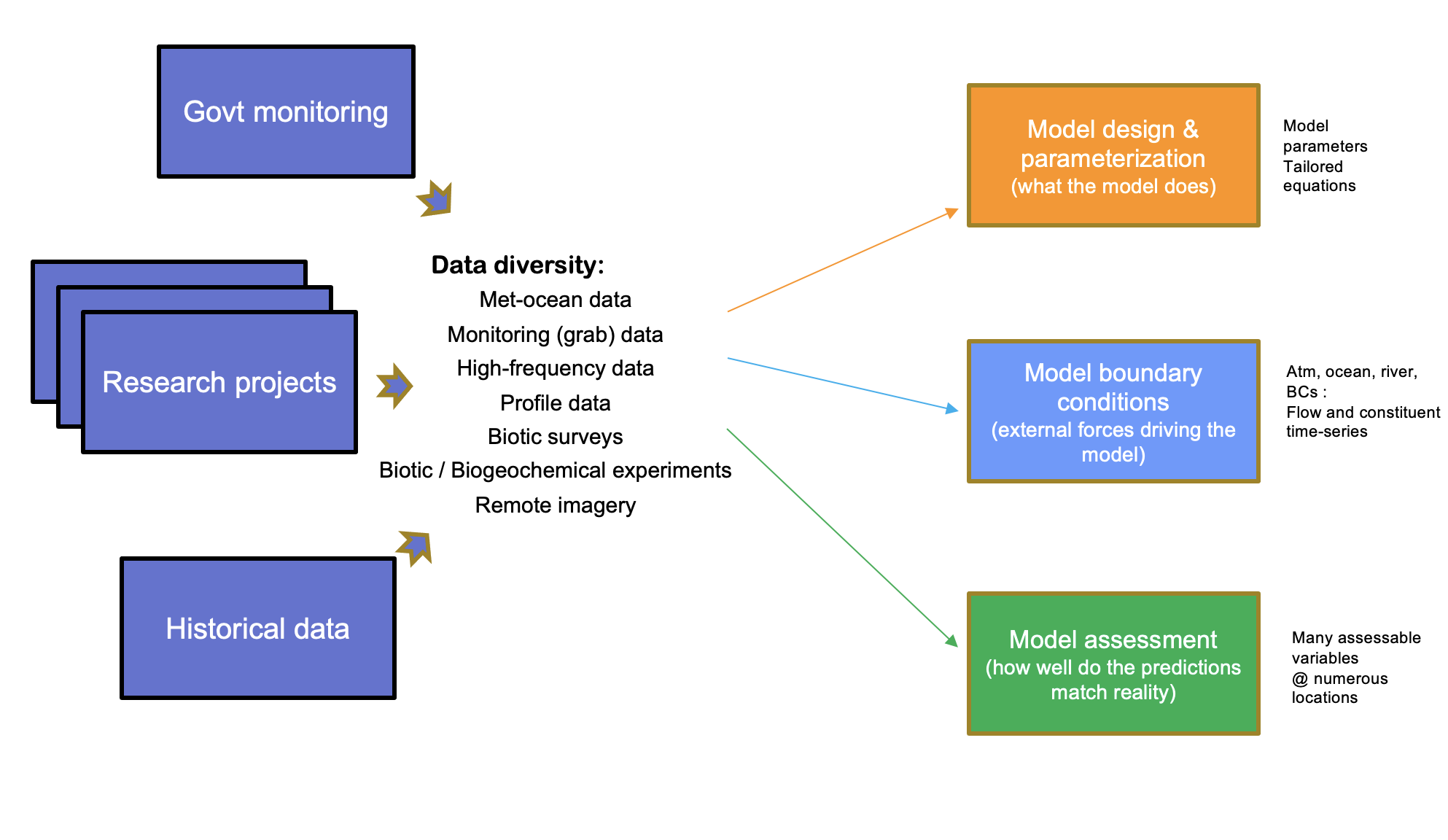
Figure 3.1: The Coorong model-data ecosystem and conceptual approach to model-data integration, accomodating data diversity and varied model requirements.

To enable the ongoing use and development of the CDM in this context, we have developed a model-data integration framework able to be used by DEW staff and project partners to co-ordinate the reference datasets needed for model development, and standardise the data integration and modelling workflows. The below sections describe how the CDM is organised, the tools and approaches used for model provenance and managing data streams, and model versioning.

3.1 CDM structure and organisation

The CDM has been designed is such a way to both facilitate the sharing of data and models across various agencies and researchers, as well as providing a formalised structure to store, catalogue and process complex and unique datasets. Comparmentalised data structures have been implemented to allow for tracking and version control of data and models as they are utilised and upgraded throughout the project.

Data cataloguing via the “CDM Data Catalogue” (described in Section 3.4) has been designed with cross-agency usage in mind. Integration with the HCHB MEK Catalogue is essential to allow for the tracking of data changes and upgrades throughout the project. The “Point of Truth,” “MEK Catalogue Classification” and “Status Notes” catagories have been included in the CDM Data Catalogue to track a dataset’s evolution throughout the project.

Github has been chosen to house the repository based on it’s mature version control systems and cross platform program support to aid all stakeholders accessing the data and models (https://github.com/). In addition, there is a wide variety of documentation online to assist users new to GitHub.

3.1.1 Online repository access

The data and model files are stored in the Github CDM Repository and shared with HCHB research partners.

3.1.2 Repository folder structure

The folders structure follows the logic of data types and resources as shown in Figure 3.2.

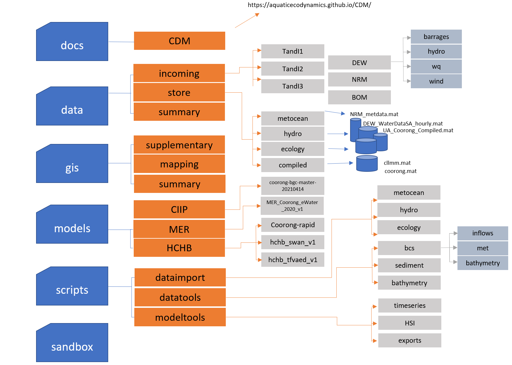
Figure 3.2: CDM online data storage folder structure

The root directories are listed and described below:

Table 3.1: CDM Root Folder Descriptions

Folder Name	Description
docs	Documentation relevent to the CDM repository (including this manual)
data	All raw & processed data, as well as summary images and tables
gis	All QGIS project files, GIS data files and summary maps and images
models	All models created and utilised during the project
scripts	All Matlab, R & Python scripts used to import & process data, as well as model creation
sandbox	All free directory users can add scratch files and temporary datasets

3.1.3 High level workflows

The raw data collected from previous works and current HCHB component outcomes are stored in the data/incoming folder and classified by their sources. These raw data are then post-processed using standard scripts (stored in the scripts folder) to convert the raw data into ‘standard’ data format (stored in the data/store folder) for model configuration, calibration/validation, and reporting (see 2.4.2 Data organisation for more details). The data-model workflow is shown in Figure 3.3.

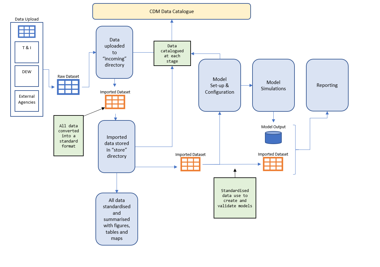
Figure 3.3: CDM conceptual diagram showing the flow of data through the system

3.2 Data repository and management

3.2.1 Data catalogue

All data that is uploaded to the CDM github repository is logged in the CDM Data Catalogue. The catalogue (found in the data directory) is comprised of a main data sheet (“CDM Data Catalogue”) as well as summary sheets for all processed data. Every raw datafile is logged with the following information:

Table 3.2: CDM Catalogue Metadata

Classification	Description
AED Classification	Description code for the data
Agency Code	Legend name for the data
Document Title	Title of Raw document, or folder name is large number of files (e.g. Year met station downloaded data)
Description	Brief description of the data
# Sites	Number of unique sites in the data
Date Range	Total date range for the data
CDM Location	Agency / Location responsible for maintaining raw data
Point of Truth	Agency / Location responsible for maintaining raw data
Contact Name	Author of Document or person responsible
Contact Email	email address of Contact Name
MEK Catalogue Classification	Location within MEK Catalogue
Status Notes	Notes on whether the dataset is finalised, or if work is ongoing
Summary Sheet	Sheet within this document summarising the data & sites
Import Status	Yes / No
Store File	Processed data file
Summary Images	Images for each site & variable
Conversion File	XLSX spreadsheet with any site name and variable conversions
GIS File	Shape file or raster
GIS Map	Final GIS map showing sites & other information
Supplemental File	store file with data merged from other uploads (coorong.mat)
BC Usage	If data is used in the creation of model BC files
Validation Usage	If data is used as part of the model validation

A catalogue of all data under management of the CDM is provided in Appendix A.

3.2.2 Data organisation

All raw data is initially uploaded into the data/incoming directory is filed under either it’s Trials and Investigations (T&I) component, or the agency responsible for supplying the data.

Data is then imported into a common format via the scripts found in the scripts/dataimport directory and stored in the data/store directory. Although some imported data may contain extra fields, all imported data contains the following fields:

Table 3.3: CDM Stored Data

Type	Description
Site Info
X	X Co-Ords of site in UTM
Y	Y Co-Ords of site in UTM
Name	Site Name
Agency	Classification code matching entry in CDM Catalogue
Data Info
Data	Array of Data Values
Date	Array of Sampling dates in Matlab Julian Date format
Depth	Array of sampling depths
Units	Data Units

Once imported, the data is then summerised via a script in the scripts/dataimport/summary directory to create a standard set of plots and summary tables that can be found in the data/summary directory. ESRI shapefiles are also automatically produced and saved into the gis/summary directory to be used to create a stardarised site map of the data’s sampling locations.

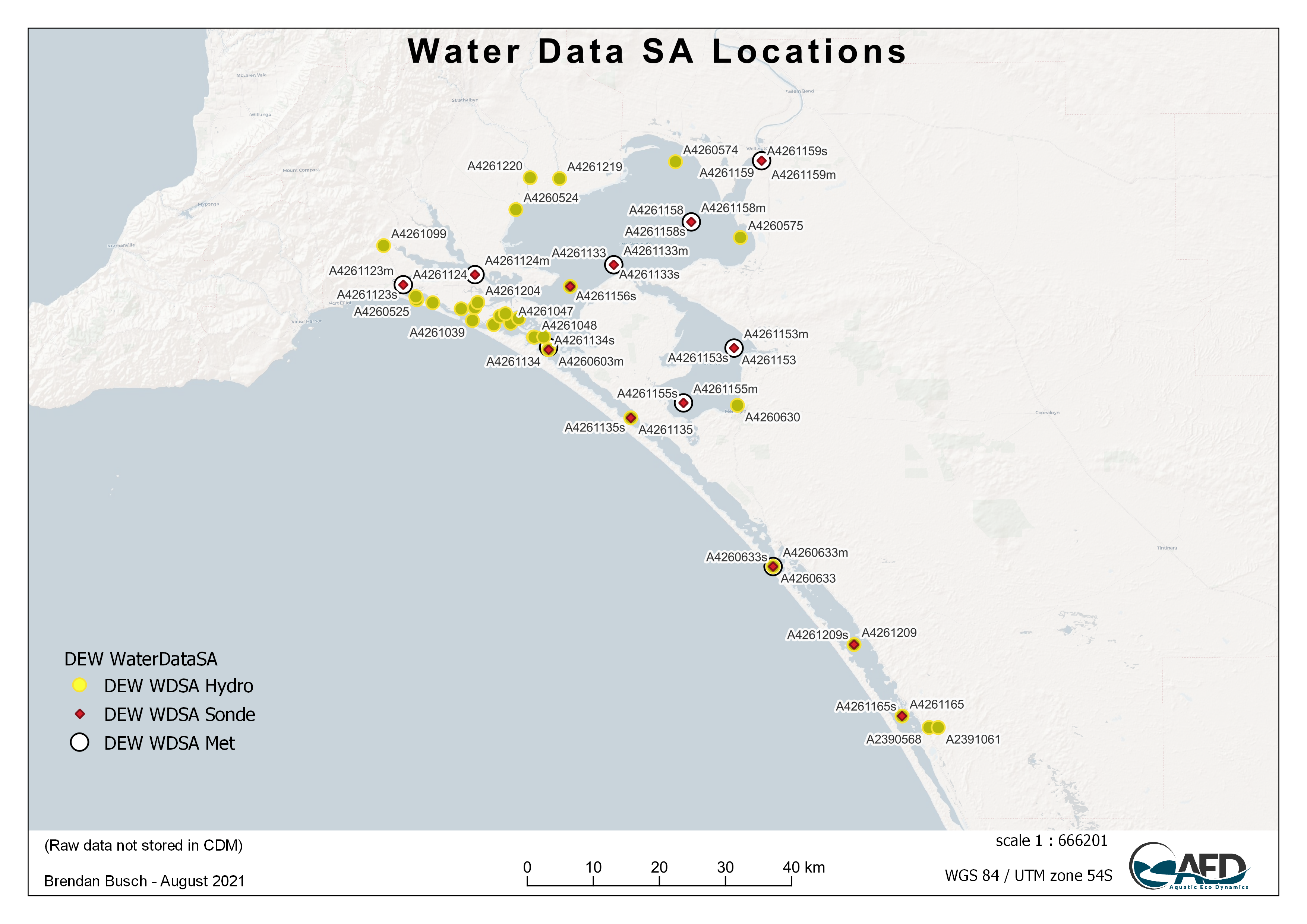
Figure 3.4: Example GIS Map showing the sampling locations for the Water Data SA online data

3.2.3 Data processing workflows

The data processing scripts for the CDM are all contained within the scripts/ directory, which has three subfodlers:

• dataimport: All scripts that import data into the CDM, or process data into a common format
• datatools: All scripts that use processed data to create additional datasets or model input files
• modeltools: All scripts that use processed data and model output to create additional datasets, model validation images and analysis

Scripting has been predominately carried out utilising the Matlab programming language, however there are scripts within the scripts directory using both R and Python. Users are able to add scripts in their preferred language; the repository core scripts for data storage and model plotting are currently in Matlab.

Below is an example workflow outlining how a meteorological boundary condition file for the TUFLOW-FV model is created (Figure 3.5. Data is first downloaded and processed by scripts in the dataimport directory. A series of Matlab functions found in the datatools directory then read in the processed data (archived in the data/store directory) and use it to create the meteorological boundary condition file for the model. Both Matlab and R scripts were used in this example.

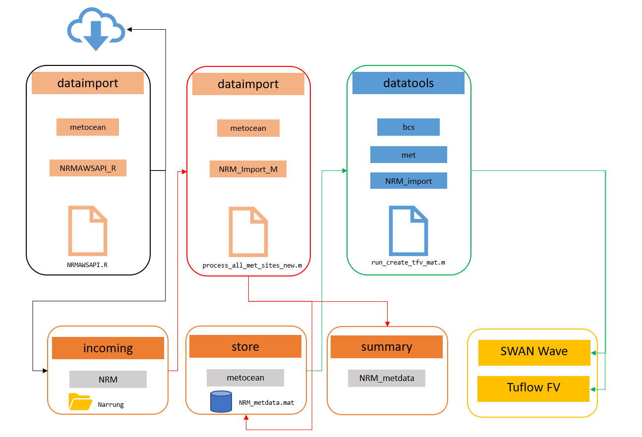
Figure 3.5: CDM work flow diagram for met data

3.3 Model repository and management

3.3.1 Model catalogue

All model files are stored in the models folder. As the model is developed over time, the model files are classified with project names and model generation identifiers. The ‘MER’ folder contains the model files used for assessing ‘eWater’ within the MER program; the ‘CIIP’ folder contains the model files developed for assessing CIIP scenarios, and the ‘HCHB’ folder contains the the core CDM files being updated throughout the HCHB project.

Models within each project directory are separated via both generation and model type. Within the HCHB model folder there are currently 4 distinct models:

• hchb_swan_v1
• hchb_tfvaed_Gen1.0_1PFT
• hchb_tfvaed_Gen1.5_4PFT_MAG
• coorong-rapid

The hchb_swan_v1 is the first generation of the Coorong SWAN Wave model that has been developed (see Section 3.2). Found inside the hchb_swan_v1 directory are two zipped model folders:

• Coorong_swn_20170101_20220101_UA_Wind_200g_2000w.zip
• Coorong_swn_20191101_20220101_UA_Wind_200g_2000w.zip

The coorong-rapid simulation folder and the hchb_tfvaed_Gen1.0_1PFT simulation folder both contain TUFLOW-FV - AED simulations, but are kept separate as they constitute different generations, using different grids, simulation periods and BC files. The Generation 1.5 simulation (hchb_tfvaed_Gen1.5_4PFT_MAG) represents an upgrade in the number of phytoplankton groups, new material zones and the addition of macroalgae.

Each model folder may contain multiple simulation sets, but they will all rely on the same model base configuration, with minor differences or adujstments. Major changes to a model’s configuration will constitute a change in generation numeber and these are stored in a separate folder. Note, models uploaded to the CDM repository may have been created by different agencies and researchers and should maintain a consistent naming convention.

3.3.2 TUFLOW-FV model organisation

Each version of TUFLOW-FV models in the CIIP and HCHB sub-folders are organised with the following structure:

• Bc_dbase (or BCs): boundary condition files, including tide and inflow boundary files; meteorological boundary files, and initial condition files;
• External: AED model files linked with the TUFLOW-FV, and optionally the ‘GOTM’ vertical mixing model if the CDM is in 3D mode;
• Model: TUFLOW-FV model structure files, including geometry and mesh files, and GIS files controlling the nodestrings and material zones;
• Run: model control/configuration files;

The TUFLOW-FV model found in the MER project folder was created prior to the above structure being implemented and contains the following folder structure:

• BCs: boundary condition files, including tide and inflow boundary files; meteorological boundary files, and initial condition files;
• External: AED model files linked with the TUFLOW-FV, and optionally the ‘GOTM’ vertical mixing model if the CDM is in 3D mode;
• GEO: TUFLOW-FV model structure files, including geometry and mesh files, and GIS files controlling the nodestrings and material zones;
• INPUT: model control/configuration files;
• Plotting : Directory to store model output images;

The hchb_tfvaed_Gen1.5_4PFT_MAG simulation folder also contains a bin directory containing the windows binaries for the TFV-AED model

• TFV: Build version: 2020.03.105
• AED: Build version: 2.0.5b

3.3.3 SWAN Wave Model organisation

The SWAN Wave models found in the HCHB model directory have the following format:

• 01_geometry : Contains the bathymetry input files as well as a automatically generated image of the bathymetry and a matlab .mat file containing the bathymetry information;
• 02_bc_dbase : Contains the processed wind input files
• 03_simulation : Contains the INPUT control file required to run the simulation
• 04_results : Model output directory

The script required to create and configure a new SWAN wave model can be found in the scripts/datatools/wave directory.

3.3.4 Model processing toolbox

The processing of any model output is predominately written and run in Matlab. Scripts that have been specifically developed for this project are contained within the scripts/modeltools directory. Scripts that have created Figures 3.9, 3.11 and 5.2 (among others) can be found here.

Plotting and model processing types include:

• Time-series plotting;
• Transect plotting;
• Model animation creation;
• Error assessment;
• Wave model plotting;
• Habitat mapping (e.g., Ruppia & Fish HSI processing and mapping)
• Scenario comparison and “DelMap” plotting;
• Nutrient budget assessments.

In particular, the publicly available GitHub repository called aed_matlab_modeltools is used and contains a wide variety of matlab scripts and functions that are frequently used to process and visualise model output. plottfv_polygon and plottfv_transect are the main functions that are frequently used. Tables 7.3 and 7.6 in Appendix B are examples of output generated via the plottfv_polygon function found in the aed_matlab_modeltools repository. This plotting function uses data and gis files stored in the CDM repository, in addition to model output to create timeseries plots of the model (averaged within a polygon region) compared against field data. The plotting function will also automatically calculate a range of error statistics based on model output and field measured data.

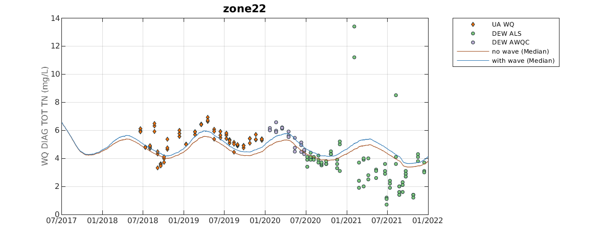
Figure 3.6: Example output from plottfv_polygon with error matrix

plottfv_transect can also be found in the aed_matlab_modeltools repository. This plots model data extracted along a transect line during a specified plotting period, and compares against the range of field data found within that period.

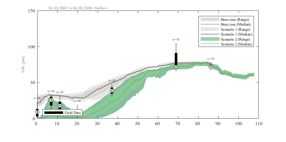
Figure 3.7: Example output from plottfv_transect with distance from Goolwa Barrage (km) along the x-axis

The aed_matlab_modeltools also houses scripts and functions for:

• Nutrient Budgeting;
• Stacked Area Transect;
• Curtain plotting;
• Mesh manipulation tools;
• Data exports;
• Sheet plotting and animation tools;

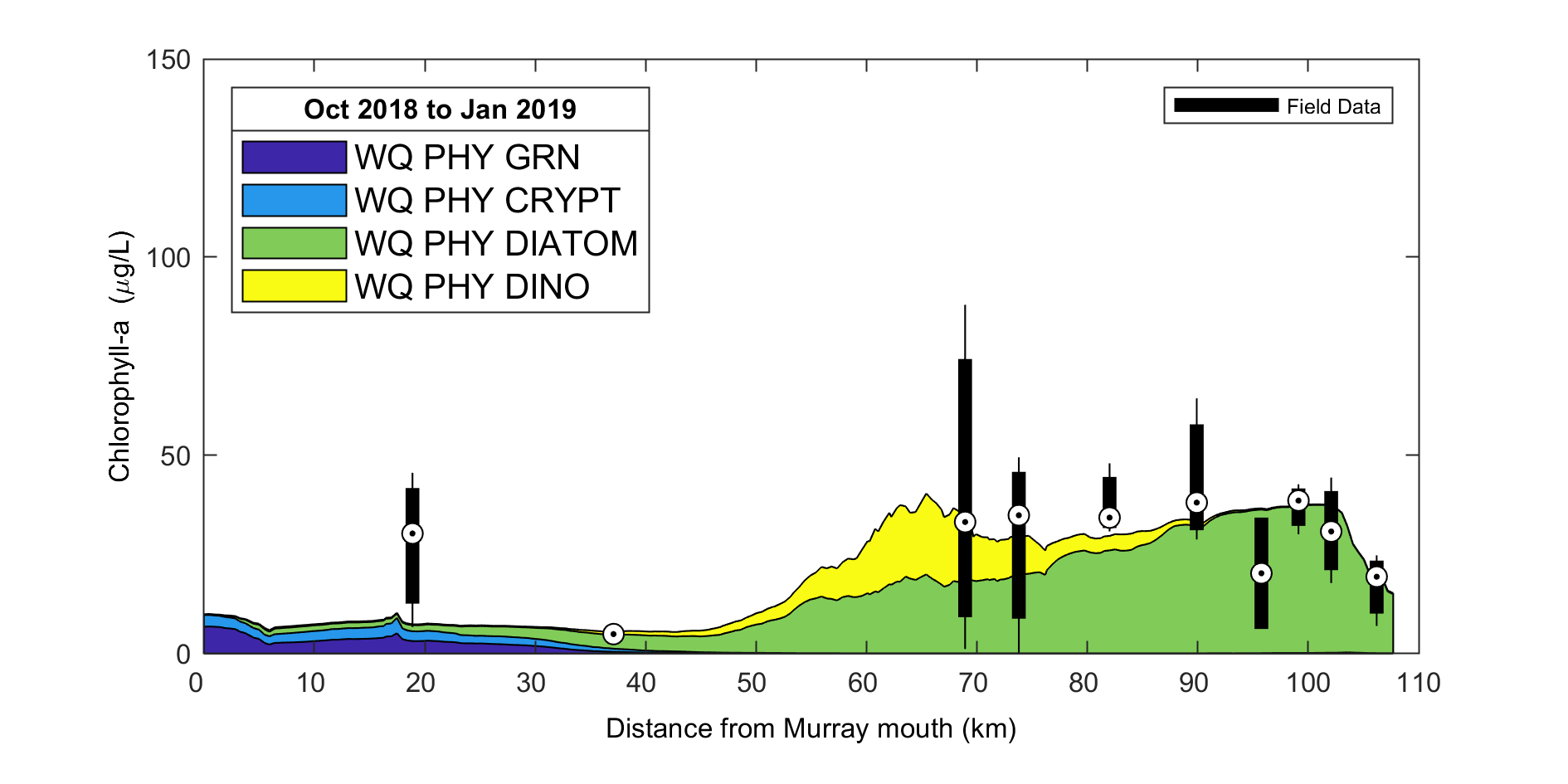
Figure 3.8: Example output from plottfv_transect_StackedArea with distance from Goolwa Barrage (km) along the x-axis

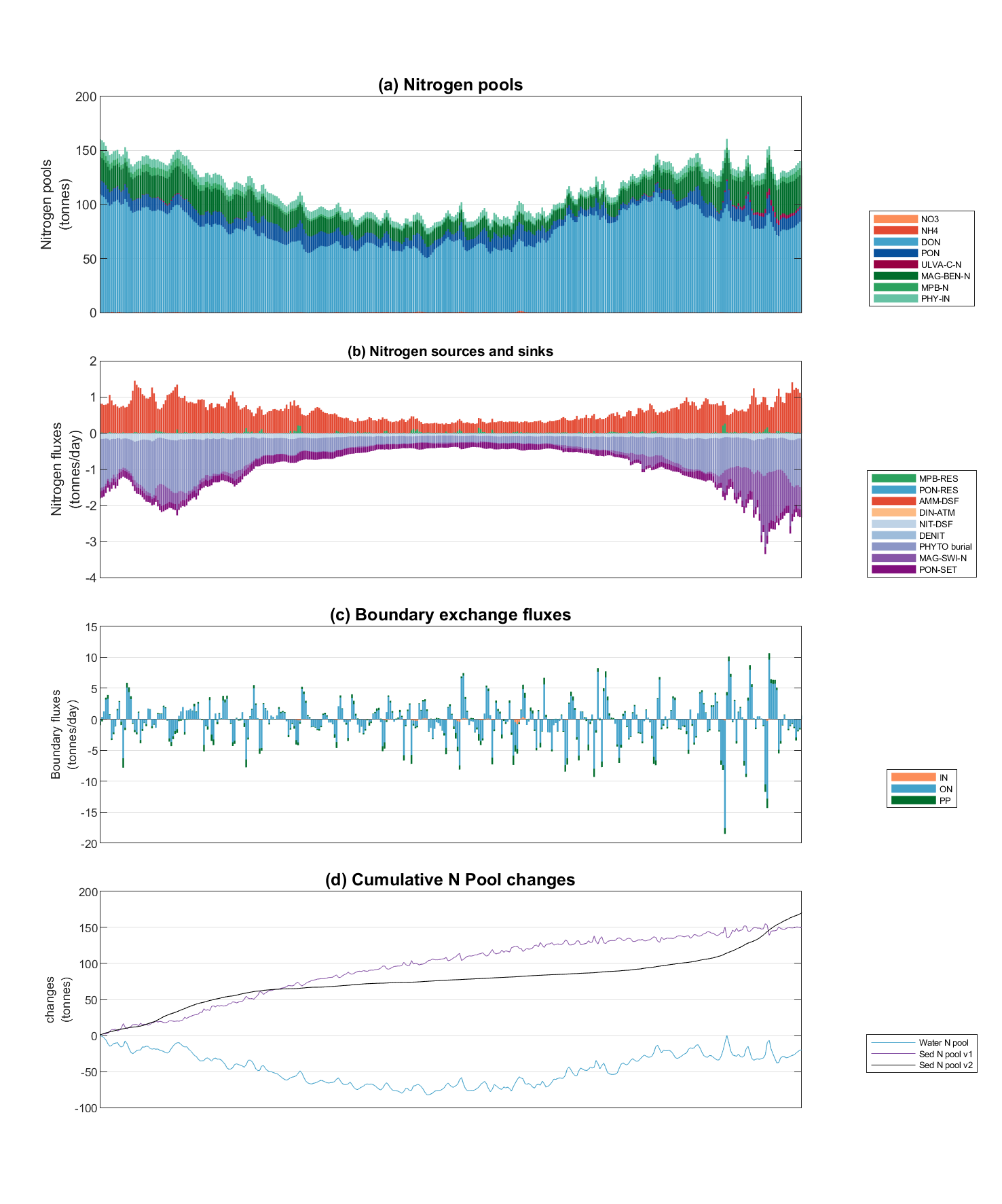
Figure 3.9: Example Nutrient Budgeting output of the North Coorong

Information on how to clone a publicly available GitHub repository can be found here.