8 Habitat Modelling
8.1 Habitat modelling - Ruppia
8.1.1 Overview
Whilst the Coorong is a naturally saline to hyper-saline lagoon, freshwater flows are important in maintaining estuarine habitat and ecosystem health and preventing extreme hyper-salinity (Brookes et al., 2009). Ruppia tuberosa is an important macrophyte in the Coorong that provides habitat for fish and food for herbivorous birds (Phillips and Muller, 2006), and it can tolerate a salinity higher than natural seawater. It therefore is known to concentrate in the mid to southern regions (Figure 8.1).
The germination and growth of R. tuberosa is known to be governed in large part by changes in salinity and water level regimes, which are influenced by flows through the barrages (Kim et al., 2013). Other factors that influence R. tuberosa growth include nutrient availability, water temperature, sediment quality and interactions with algae, including shading of light and interference with flowers and fruits on the surface. Early summer flows are thought to be particularly beneficial as they delay the drop in water level in the South Lagoon and can prevent extreme salinities emerging, thereby encouraging a more complete reproductive cycle (Collier et al., 2017).
In addition, salinity has also been identified as the key driver that influences fish assemblage structure and the extent of estuarine fish habitat in the Coorong (Ye et al., 2011). This section describes how simulations of Ruppia and estuarine fish habitat have been configured and assessed.
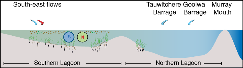
Figure 8.1: Conceptual diagram of Ruppia presence in the Coorong, under base case conditions= with moderate inflows from the Barrages (North) and Salt Creek (South-east).
8.1.2 Model description: Ruppia HSI
The approach adopted in the current study is to simulate “habitat suitability” based on an assessment of modelled environmental conditions relative to the known requirements of Ruppia tuberosa, for example, considering salinity, light and/or other environmental conditions. This approach was then used to define a relative index for each computational cell by overlaying the various environmental controls/limitations that have been informed based on prior experiments and surveys. The Habitat Suitability Index approach empirically defines conditions that lead to successful growth and reproduction, without simulation of processes such as photosynthesis and respiration.
For the Coorong, a similar habitat model approach was undertaken previously by Ye et al. (2014), who focused exclusively on the salinity and water level requirements of Ruppia and presented the model results as an overall probability that Ruppia plants would successfully complete their lifecycle, by accounting for the different tolerances of different life stages.
In this study, we used the hydrodynamic-biogeochemical model to predict environmental conditions at high spatial and temporal resolution for a period of multiple years, and used this to calculate the habitat suitability index (HSI) for each particular phase of the life cycle of Ruppia (Figure 8.2). The calculation of the HSI required the integration of environmental conditions over a biologically relevant time period, based on the typical duration and seasonal timing for each life-stage. HSI results for different life stages were then combined and integrated to obtain overall HSI results for successful completion of sexual or asexual life cycles of Ruppia. For each annual cycle these model results were then summarised over the length of the Coorong, to allow estimation of the total suitable area.
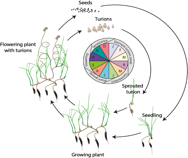
Figure 8.2: Overview of the sexual and vegetative life cycles of Ruppia tuberosa (from Collier et al. 2017).
Ruppia Habitat Suitability Index calculation
In each model cell (\(c\)), the Habitat Suitability Index (HSI) is computed based on suitability of conditions (\(i\)), for each of the main life-stages (\(j\)), by defining a fractional index, \(Φ\). The fractional index for each attribute is computed at each time, step and then integrated over a time window, specific to the life-cycle stage.
\[ \Phi^{HSI_{j}}_{i} = \frac{1}{t_{j_{\text{start}}}-t_{j_{\text{end}}}} \sum^{t_{j_{\text{end}}}}_{t=t_{j_{\text{start}}}}\Phi^{HSI_{j}}_{i}(i)_{t} \tag{8.1} \\ \scriptsize{ \\ \text{whereby: $i$ = {salinity, temperature, light, depth, algae}} \\ \text{and: $j$ = {seed, sprout, adult, flower, turion} (Generation 0), or} \\ \text{$j$ = {turion viability, seed, sprout, adult, flower, turion} (Generation 2.0)}} \]
The integration time for each life-stage, \(j\), is selected from within the available plant growth windows, as indicated in Table 8.5 (Generation 0) and Table 8.7 (Generation 2.0).
The above function is computed in each cell and produces maps of suitability (between 0 and 1) for each environmental attribute for each life stage within any given year. The individual functions are piece-wise, based on synthesis of the available literature and analyses of survey data (Table 8.1). These are then overlaid to produce a final map for any given year using:
\[ \Phi^{HSI}_{c} = \text{min}\left[\Phi^{HSI_{j}}_{i} \right]_{c} \tag{8.2} \]
To compare the overall area of suitable habitat between years, or the relative suitability of alternate scenarios, the fractional suitability is used as a multiplier with the cell area, according to:
\[ A^{HSI} = \sum_{c} \Phi^{HSI}_{c} A_{c} \tag{8.3} \]
and the spatially averaged HSI in any given region (with area A) is computed as:
\[ \overline{HSI} = \frac{1}{A}\sum_{c} \Phi^{HSI}_{c} A_{c} \tag{8.4} \]
8.1.3 Data availability
The model approach requires empirical data for a) assignment of appropriate environmental threshold data for each life-stage, and b) validation and assessment of the approach under various conditions. The available data for this tasks is described next.
8.1.3.1 Environmental threshold review
Ruppia life-stages
Ruppia life-stage time windows were reviewed based on both the phenology and seasonal survey datasets collected during the HCHB program. Number of Ruppia flowers, fruits, seeds, turions and their biomass recorded at each site during September 2020 – December 2021 as well as algae biomass were grouped by month and plotted as timeseries to visualise the peak of life-stage events that are relevant to the Ruppia habitat model. It was evident that the peak of flowering/fruiting and turion formation lies between September and December (Figure 8.3 and Figure 8.4). Seed count peaked around March – May in 2021, as well as during the reproductive period (September – December) in 2020, however in 2021 Dec much fewer seeds were recorded (Figure 8.3). Peak algae growth occurred around September – December, coincident with the Ruppia reproductive period (Figure 8.5). It was suggested that there were remnant living plants during the aestivation season (January – March), which indicates the presence of a perennial Ruppia community (Lewis et al., 2022).
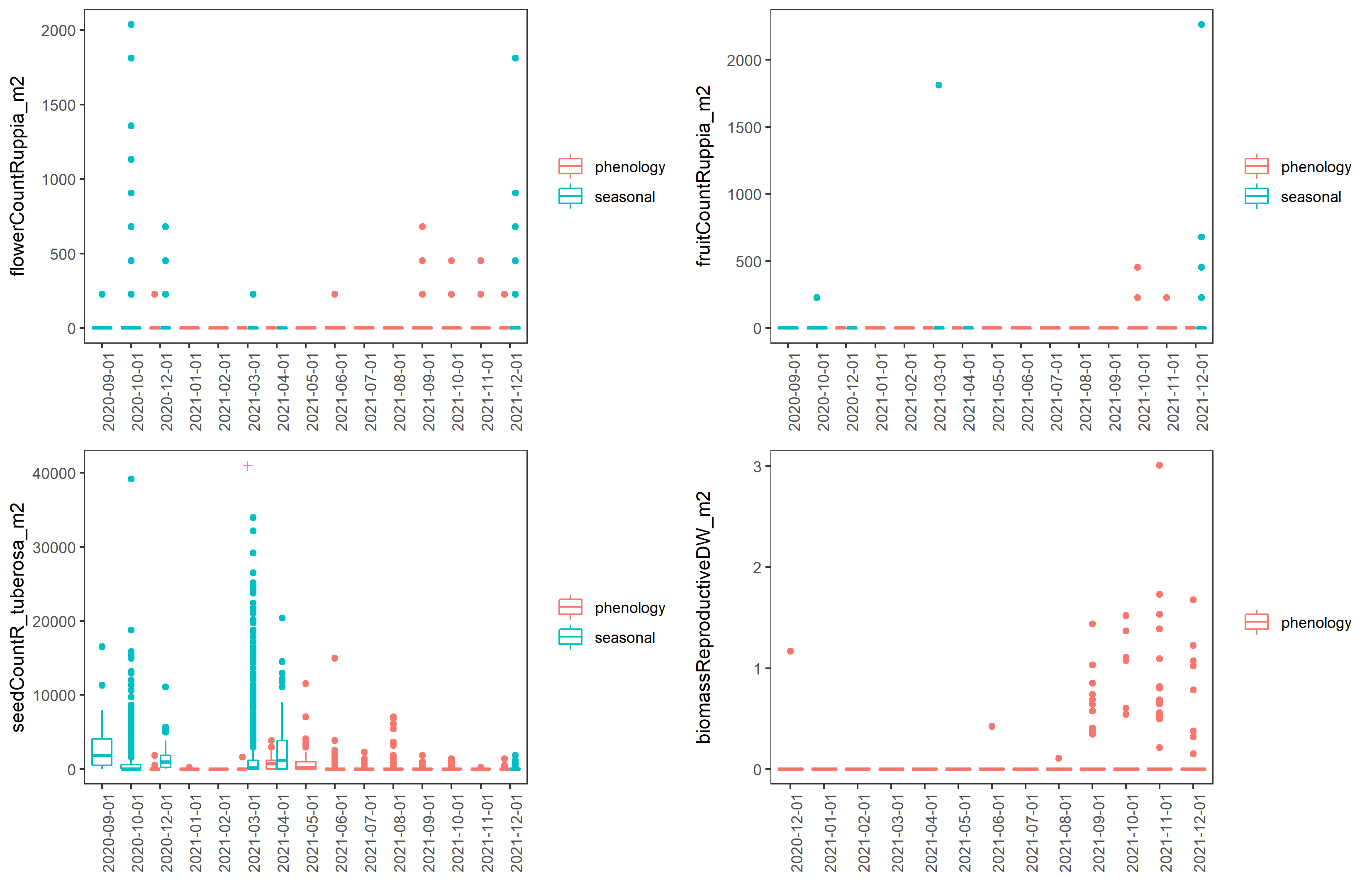
Figure 8.3: Boxplots of monthly Ruppia flower count, fruit count, seed count (per m2) and biomass of sexual reproductive structures (inflorescence, flowers, fruits, g DW/m2) between December 2020 and December 2021. ‘+’ indicates data outside of plotting range.
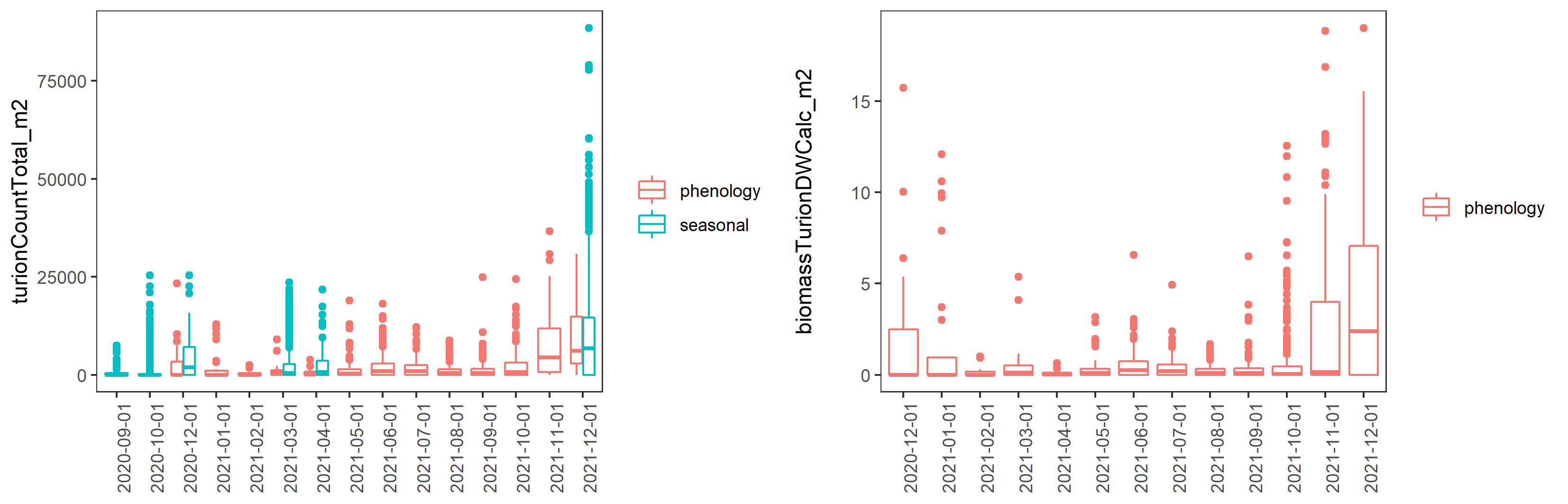
Figure 8.4: Boxplots of monthly Ruppia turion count (type I and type II combined, per m2) and turion biomass (type I and type II combined, g DW/m2) between December 2020 and December 2021.
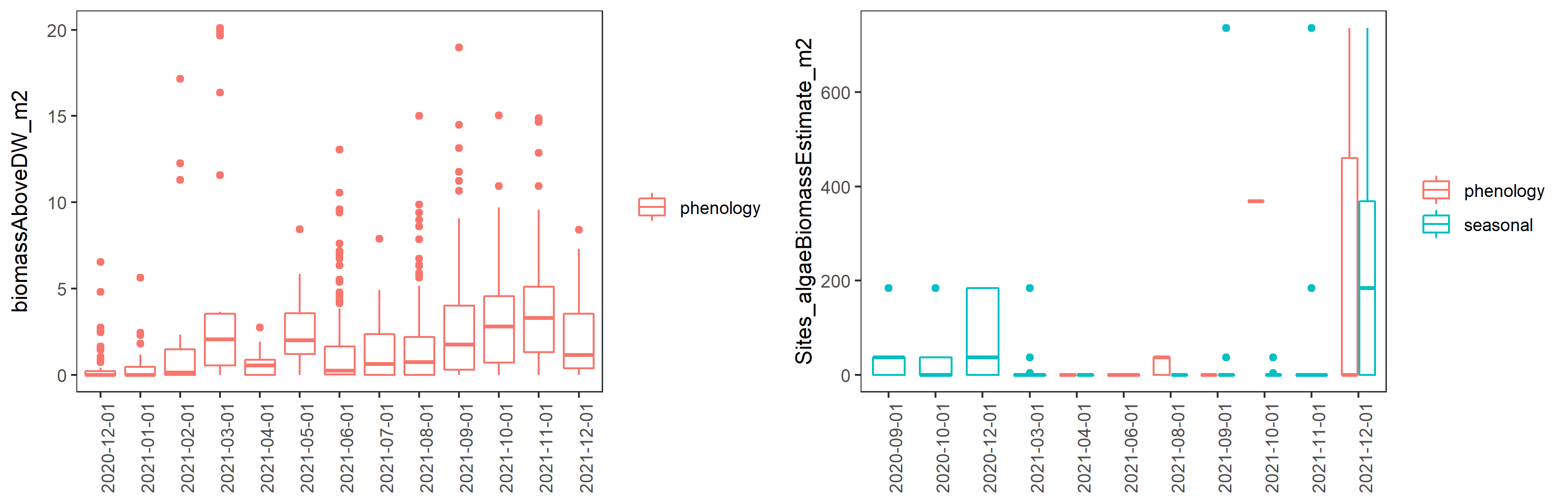
Figure 8.5: Boxplots of monthly aboveground macrophyte biomass (excluding reproductive structures, g DW/m2) and estimated algae biomass (g DW/m2) between December 2020 and December 2021.
Environmental threshold parameters
Environmental conditions and thresholds suitable for Ruppia growth, including salinity, water depth, light availability and temperature have been reviewed and summarised in Table 8.1 based on existing literature and analyses of survey data collected during the HCHB program.
| Environmental condition | Thresholds | Rationale | Source | Comment |
|---|---|---|---|---|
| Turion viability (Jan 1 – Mar 31) | ||||
| f(S): Salinity (g/L) |
<135 optimal 135–165 suboptimal >=165 unsuitable |
Turions once formed will lose viability to high salinities (more vulnerable than seeds) during summer dormancy period. Experiments showed that after 60 days of treatment in salinities of 135 – 180 g/L, only 5 – 10% turions sprouted when transferred back to salinities below 120 g/L. Turions only sprouted in 0 g/L (which is unlikely to occur in Ruppia habitat in the lagoon) after salinity treatment at 165 g/L. |
Kim et al. (2013); Kim et al. (2015) |
A new function in Gen II model |
| Seed germination (Apr 1 – Jun 30) | ||||
| f(S): Salinity (g/L) |
0.1-40 optimal 40-85 suboptimal >85 unsuitable |
R. tuberosa seeds with sediment germinated in salinities of 0 to 85g/L with 14-64% germination, but no germination occurred above 85g/L. R. tuberosa seeds without sediment germinated in 0 - 90g/L. In salinity below 40g/L a germination probability of >50% would be expected for seeds of R. tuberosa, but at salinities between 40 and 90 g/L germination would be<50% | Kim et al. (2013) | - |
| Turion sprouting (Apr 1 – Jun 30) | ||||
| f(S): Salinity (g/L) |
<=0.1 unsuitable 0.1-20 suboptimal 20-75 optimal 75-125 suboptimal >125 unsuitable |
Turions of R. tuberosa germinated at salinities of 0 to 125g/L, with 14 - 74% germination, but no germination occurred above 125 g/L. Suboptimal thresholds based on Fig.2 in@kim2013 |
Kim et al. (2013); Asanopoulos and Waycott (2020) Fig.5 |
- |
| Adult plant growth (Jun 1 – Sep 30) | ||||
| f(S): Salinity (g/L) |
<10 unsuitable 10-19 suboptimal 19-124 optimal 124-230 suboptimal >230 unsuitable |
A primary factor driving the distribution and abundance of Ruppia in the southern Coorong. The highest abundance of R. tuberosa found at salinities from 19 to 70 g/L and declined sharply in response to increasing salinity from 70 to 109 g/L, but increased again between 116 and 124 g/L. Table 2 in Collier et al. 2017 indicated R. tuberosa occurred at up to 230 g/L in other Lakes but source of data is not clear. Lower threshold source based on Fig.5 in Asanopoulos and Waycott (2020) |
Brock (1982); Kim et al. (2015); Collier et al. (2017); Asanopoulos and Waycott (2020) |
The model relating shoot density to physicochemical conditions explained 73% of variation (Kim et al. 2015) |
| f(WL): Water depth (m) |
< 10 % of time wet: unsuitable >= 10 % of time wet: suitable |
Water depth needs to be sufficient to cover plants during growth. |
Kim et al. (2015); Collier et al. (2017) |
Shoot abundances were observed to be highest at water depths between 0.2 and 0.6 m in Coorong. However this depth preference is likely the result of trade-off between light requirement (thresholds included in f(l)) for photosynthesis and preventing desiccation. |
| f(l): Light (%SI) |
<=5 unsuitable 5-36 suboptimal >=36 optimal |
There was a significant (p <0.001) effect of the light treatment on biomass of R. tuberosa after 8 weeks of shading. Biomass was significantly reduced in the 5% light treatment compared to the 36, 63, 86 and 100% light treatment. | Collier et al. (2017) cited in Asanopoulos and Waycott (2020) | - |
| f(T): Temperature (°C) |
<4 unsuitable 4-10 suboptimal 10-23 optimal 23-30 suboptimal >30 unsuitable |
The optimum temperature for photosynthesis of Ruppia sp. is approximately 20 – 23°C. At temperatures that are =30°C biomass declines, and if sustained, there may be no reproductive output. Lower threshold is unclear | Santamarı́a and Hootsmans (1998) cited in Collier et al. (2017). | The optimum is not specifically for R. tuberosa. |
|
f(FA): Algal biomass (g DW/m2) |
<=100 optimal 100-368 suboptimal >368 unsuitable |
Surface mats formed by the filamentous algae shade submerged plants and entangle flowers/fruits, causing them to break away from stems before they mature. It was suggested that to maintain and improve the condition and resilience of the Ruppia community, algal mat formation should be reduced to less than 100 g/DW per m2. Upper thresholds derived from analysis of HCHB survey data (Figure 8.9) | Lewis et al. (2022) | - |
| Flowering and seed set (Sep 1 – Dec 31) | ||||
| f(S): Salinity (g/L) |
<12 unsuitable 12-47 suboptimal 47-62 optimal 62-100 suboptimal >100 unsuitable |
Flower abundance was highest at salinities between ~47 and 62 g/L and flower abundance was lowest at >70 g/L and <47 g/L. The highest seed density was maintained at salinities of 26–62 g/L. Upper and lower thresholds were based on Collier et al. 2017 and Fig.5 in Asanopoulos and Waycott (2020). Original source unclear |
Kim et al. (2015); Collier et al. (2017); Asanopoulos and Waycott (2020) |
The model relating flower density to physicochemical conditions explained 76% of variation but only 27% of the seed abundance variance was explained (Kim et al. 2015). |
| f(WL): Water depth (m) |
<0.01 unsuitable 0.01-0.1 suboptimal 0.1-0.4 optimal 0.4-0.9 suboptimal >0.9 unsuitable |
R. tuberosa flowers need to reach the water surface for pollination. The highest density of flowering has been observed in water depths from 0.1 to 0.4 m and seed density of mature plants declines at depths greater than 0.4 m. Upper thresholds based on Fig.4 in@kim2015. |
Kim et al. (2015); Collier et al. (2017); |
Upper threshold for seed production is 0.8m (>0.8m unsuitable) but only 27% of the seed abundance variance was explained (together with salinity), therefore thresholds for flowering was adopted here |
|
f(FA): Algal biomass (g DW/m2) |
<=100 optimal 100-184 suboptimal >184 unsuitable |
Surface mats formed by the filamentous algae shade submerged plants and entangle flowers/fruits, causing them to break away from stems before they mature. It was suggested that to maintain and improve the condition and resilience of the Ruppia community, algal mat formation should be reduced to less than 100 g/DW per m2. Upper thresholds derived from analysis of HCHB survey data (Figure 8.9) | Lewis et al. (2022) | - |
| Turion formation (Sep 1 – Dec 31) | ||||
| f(S): Salinity (g/L) |
<40 unsuitable 40-70 suboptimal 70-160 optimal 160-230 suboptimal >230 unsuitable |
Thresholds were determined considering several sources: 1) The highest turion densities in the Coorong have been observed at salinity between ~124 g/L and 160 g/L and are most likely to occur where salinities are over 70 g/L. This study was conducted during a year with extremely high salinities in the Coorong; 2) Analysis of 2020 – 2021 HCHB survey data indicates high turion abundance between ~70 – 120 g/L but can occur in salinity at as low as ~40g/L (Figure 8.6); 3) Upper threshold based on Fig.5 in Asanopoulos and Waycott (2020) |
|
|
| f(WL): Water depth (m) |
< 10 % of time wet: unsuitable >= 10 % of time wet: suitable |
Desiccation during the reproductive window (spring/summer) prevents turion production, reducing the regeneration of the population in subsequent growing seasons. |
Kim et al. (2015); Collier et al. (2017); Asanopoulos and Waycott (2020) |
Highest densities of turions were observed in 0.1–0.4 m water depths. However this depth preference is likely the result of trade-off between light requirement (thresholds included in f(l)) for photosynthesis and preventing desiccation. |
Statistical analyses were conducted on HCHB Ruppia survey data to
investigate the influences of salinity and water depth on Ruppia
abundance during 2020 – 2021, in order to further refine environmental
thresholds in the Ruppia model. This is because some of the optimal
values presented in the literature prior to HCHB were thought to be
possibly biased due to extreme environmental conditions in the Coorong
during the survey (e.g. salinity thresholds for turion formation from
(Kim et al., 2015), pers. comm). Nonparametric multiplicative regressions (NPMR,
McCune (2006)) were used to derive optimal fit models describing the
response of different life-stages of Ruppia to salinity and water
depth in seasons appropriate for each life-stage. Salinity and water
depth were found to be the most important abiotic factors influencing
the distribution and abundance of R. tuberosa in previous studies
(Kim et al., 2015). Although recent studies suggested that Distance from Murray
Mouth (DFMM), elevation and algal biomass also influence macrophyte
communities in the lagoon (Lewis et al., 2022), they are not included in this
NPMR analysis as 1) the mechanisms underlying how DFMM influences
macrophyte abundance is unclear; 2) elevation was recorded as a more
permanent landmark which does not vary between seasons compared to water
depth, however it is the actual water depth that influences the
distribution of seagrass; 3) algae biomass is also influenced by
salinity therefore co-correlation likely exists. The analysis was
conducted in R using the ‘ngnn’ package and results are shown in (Figure
8.6 and Figure 8.7) and Table
8.2 below. The abundance of Ruppia flower, seed and
macrophyte shoot recorded during 2020 – 2021 surveys in relation to
salinity and water depth largely agreed with existing literature (Table
8.1). However, relatively high turion abundance was
found to be in lower salinity conditions than previously recorded by
Kim et al. (2015). During 2020 – 2021, considerable number of turions occurred
below salinity of 70 g/L down to approximately 45 g/L, especially when
water depth <0.4m (Figure 8.6), while Kim et al. (2015)
suggested that turions were most likely to occur with salinity >70 g/L.
This finding was therefore incorporated into the turion formation
thresholds in the habitat model (Table 8.1).
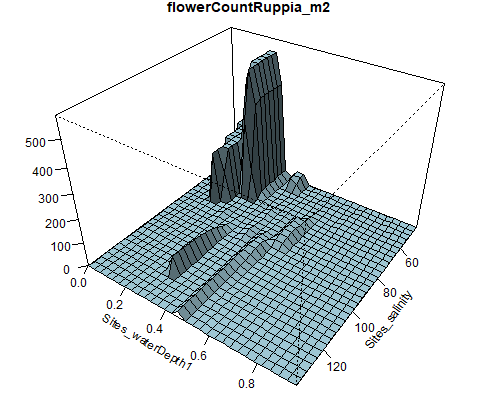
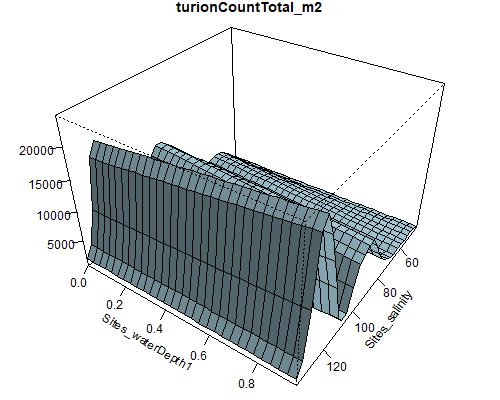
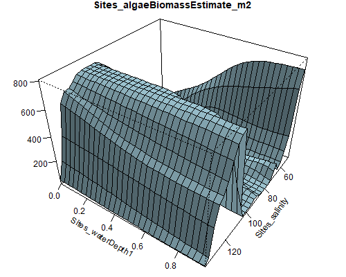
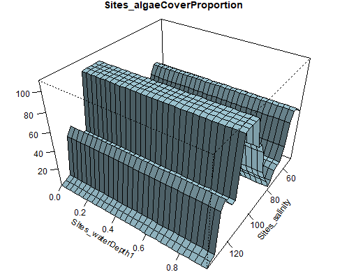
Figure 8.6: Relationship between abundance of Ruppia flowers, turions, macroalgae and salinity (g/L) and water depth (m) during the Ruppia reproductive period (Sep – Dec 2020 and Dec 2021) in the Coorong.
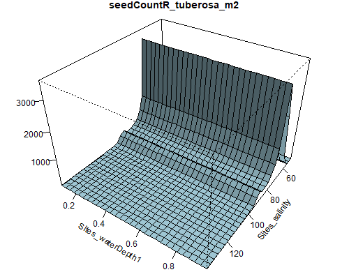
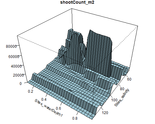
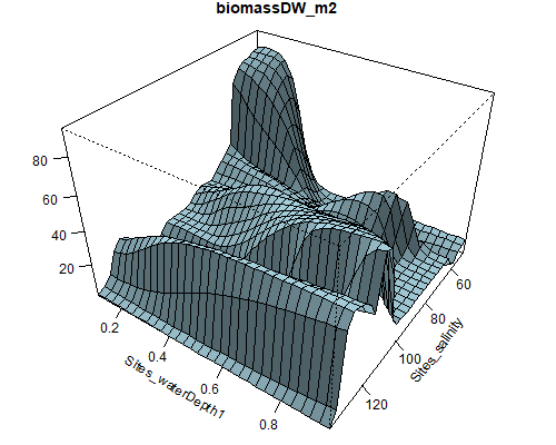
Figure 8.7: Relationship between abundance of Ruppia seeds, macrophyte shoots, macrophyte biomass and salinity (g/L) and water depth (m) during the Ruppia reproductive and aestivation period (Sep – Dec 2020, Mar – Apr 2021 and Dec 2021) in the Coorong.
| Field data | Period | R2 | Tol-salinity | Sens-salinity | Tol-depth | Sens-depth |
|---|---|---|---|---|---|---|
|
Seagrass shoot count (all spp.) |
Sep - Dec 2020, Mar - Apr 2021, Dec 2021 |
0.722 | 0.401 | 3.388 | 0.029 | 1.911 |
|
Seagrass biomass (all spp.) |
Sep - Dec 2020, Mar - Apr 2021, Dec 2021 |
0.250 | 3.147 | 3.517 | 0.074 | 3.356 |
|
Flower count (Ruppia) |
Sep - Dec 2020, Dec 2021 |
0.954 | 3.194 | 0.271 | 0.006 | 0.601 |
|
Seed count (R. tuberosa) |
Sep - Dec 2020, Mar - Apr 2021, Dec 2021 |
0.275 | 2.173 | 1.944 | 181846.000 | 1.565 |
|
Turion T1 & T2 count (Ruppia) |
Sep - Dec 2020, Dec 2021 |
0.264 | 3.784 | 2.545 | 0.346 | 2.346 |
| Algae cover % |
Sep - Dec 2020, Dec 2021 |
0.440 | 1.812 | 3.620 | 1058132.000 | 2.628 |
| Algae biomass |
Sep - Dec 2020, Dec 2021 |
0.549 | 2.667 | 3.463 | 0.123 | 2.628 |
Macroalgae influences
As the presence of filamentous algae mats is thought to negatively impact Ruppia growth by shading submerged plants and entangle flowers/fruits potentially causing sexual reproductive failure (Asanopoulos and Waycott, 2020; Paton et al., 2018), a literature review and statistical analyses on HCHB survey data were conducted on the relationship between Ruppia abundance and macroalgae abundance in an attempt to quantify the effect of macroalgae on Ruppia and improve model accuracy. Very limited literature exists on the impact of macroalgae on seagrass that may potentially be translated to the Ruppia model. A field experimental study by Bittick et al. (2018) on the effect of Ulva biomass on Zostera marina shoot density and growth indicated that Zostera shoot density was negatively affected by Ulva biomass predictable by an exponential decay function (Figure 8.8, while Zostera growth was not affected. Irlandi et al. (2004) found that 100% drift algal cover for 2-3 months produced around 25% reduction in above ground seagrass biomass (Thalassia testudinum). However, below-ground biomass, shoot density or growth rate were not impacted.
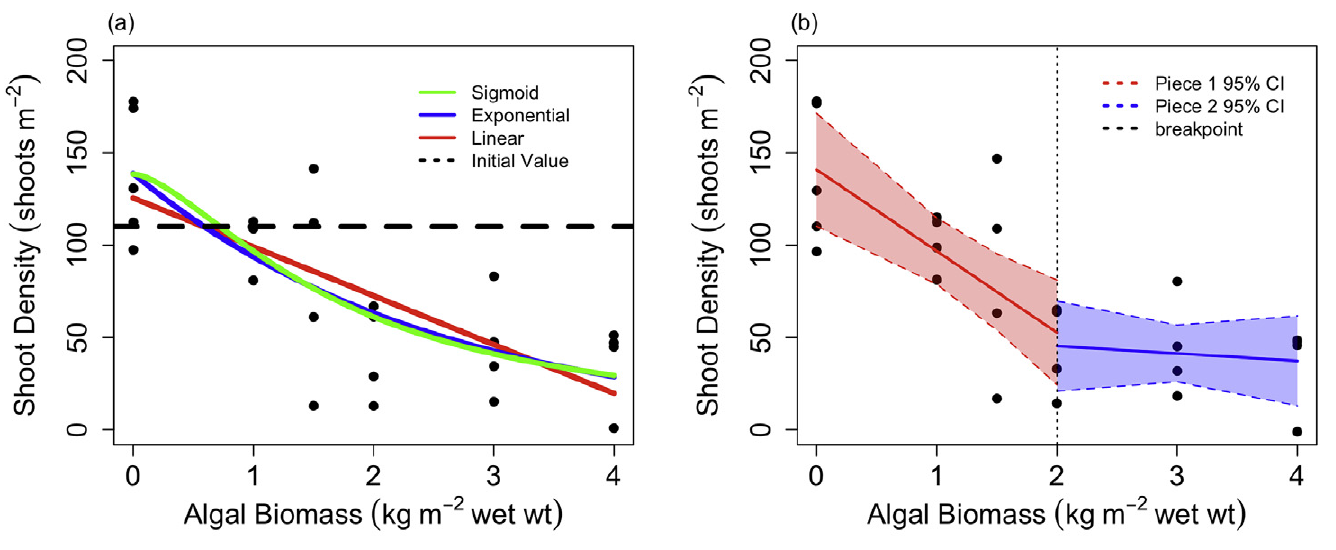
Figure 8.8: Relationship between Ulva biomass and Zostera marina shoot density (Source: Bittick et al. 2018).
During the HCHB survey filamentous algae largely co-occur with Ruppia communities both spatially and temporally, and dense mats were observed to be almost exclusively associated with the presence of macrophytes (Lewis et al., 2022). Lewis et al. (2022) identified that when estimated algae biomass exceeded 184 g DW/m2, there was a significant reduction in macrophyte biomass.As it was previously speculated that filamentous algal mats may have a negative impact on the reproductive success of Ruppia by entangling and breaking flower stalks away from the stem (Asanopoulos and Waycott, 2020; Paton et al., 2018), further analyses were conducted on the relationship between algae biomass and various Ruppia life-stages to provide insights on assigning appropriate threshold values to each Ruppia life-stage in the habitat model. HCHB seasonal survey core data including seagrass biomass, seagrass shoot count, Ruppia flower count and total turion count during period when algae growth was most active (i.e., September - December 2020 and December 2021, Figure 8.5) were averaged by site and summarised in boxplots against six levels of algae biomass (estimated by converting algal severity index, conversion method is described in Lewis et al. (2022)). Results indicated that compared to overall macrophyte biomass or density, flower density appeared to have a shaper reduction as algae biomass reached 184 g DW/m2 (Figure 8.9). Although this association may not indicate causation, a lower maximum tolerance on algae was assigned to the flowering stage than adult growth stage in the habitat model (Table 8.1) based on the assumption that the impact of dense algal mats is likely to be greater on the sexual reproductive success than on vegetative growth. In contrast, turion density appeared to be almost unaffected by high algae biomass (Figure 8.9). However, it is unclear whether this was a shift of reproductive strategy from aboveground (flowering) to belowground (turion) when algae mats were dense, or other co-correlating factors were at play. As a result, no threshold values were assigned for turion formation in the model.
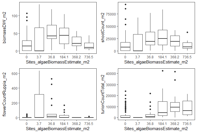
Figure 8.9: Boxplots for macrophyte biomass, macrophyte shoot count, Ruppia flower count and turion count against six levels of estimated algae biomass during September - December 2020 and December 2021.
8.1.3.2 Ruppia extent within the lagoon
The distribution and abundance of Ruppia has been regularly monitored in the Coorong since 1998. However, the types of data collected, the sampling season, location and methods varied between programs. An overview of the available historical and HBHC datasets is shown in Figure 8.10.
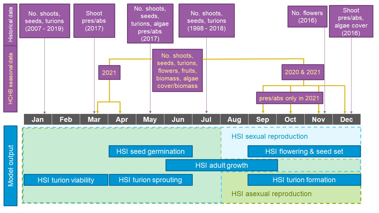
Figure 8.10: Overview of Ruppia survey datasets showing sampling periods and types of data collected (purple boxes, with HCHB data highlighted in yellow), versus habitat model output (HSI, blue boxes) on a timeline. For model output, life-stages involved in the integration of overall sexual reproduction success are shaded in light blue (with light blue dashed outline), and life-stages involved in the integration of overall asexual reproduction success are shaded in light green (with green dashed outline). Please note that the integration method shown reflects the updated Ruppia model (Generation 2.0), for detailed information on the differences between Generation 2.0 model and Generation 0 model (pre-HCHB) please refer to Section 8.1.4.
Historical Monitoring A summary of historical Ruppia monitoring
datasets (pre-2020) is shown in Table 8.3. Locations of
sampling sites are shown in Figure 8.11.
| Agency/program | Data description | Date range | No. sites |
|---|---|---|---|
| UA MDBA_1 |
No. shoots (green/brown), No. turions (half/full), No. seeds, % grazed, grazed length, presence/absence of algae, water depth (categorical) |
2017 May | 8 |
| UA MDBA_2 |
No. shoots (green/brown), No. turion (type I/II), No. seeds |
1998 – 2018 every Jul | 13 |
| UA MDBA_3 | No. flowerheads | 2016 Nov | 9 |
| UA MDBA_4 |
No. shoots (green/brown), No. turions (type I/II), No. seeds, No. flower stalks (since 2017, limited sites only), % grazed, grazed length, water depth (categorical) |
2007 – 2019 every Jan | 22 |
| UA ORH |
presence/absence of Ruppia, algae No/Rare/Present/Extreme, water depth, salinity |
2016 Dec, 2017 Mar |
24, 11 |
| UA |
No. shoots, % cores with shoots |
1999 – 2015 every Jul | 13 |
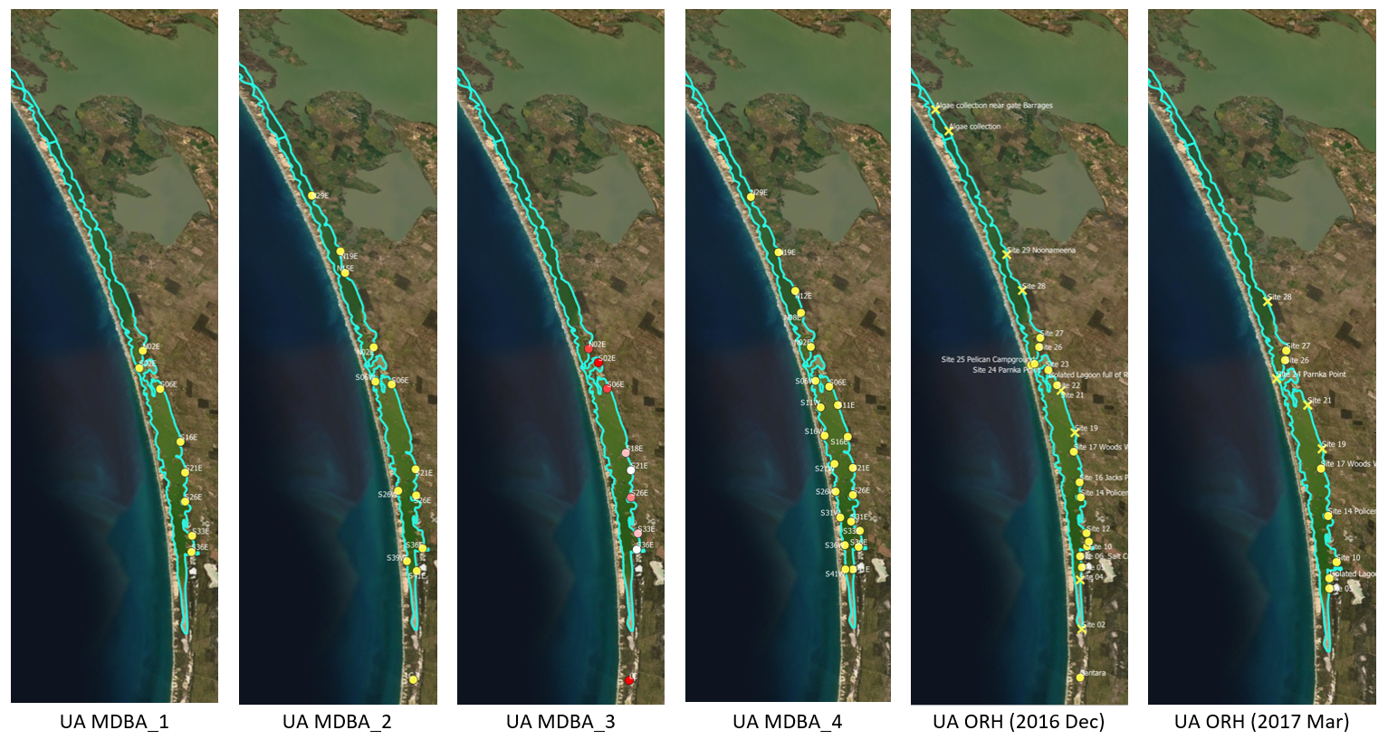
Figure 8.11: Ruppia sampling sites for various monitoring program prior to 2020. Agency/program code under each map corresponds to those listed in Table 8.3. Turquoise outline represents the model boundary. Note that sampling sites of the last dataset listed in Table 8.3 are the same as UA MDBA_2.
HCHB Monitoring A summary of the HCHB monitoring datasets is shown
in Table 8.4. Locations of sampling sites are shown in
Figure 8.12.
| Agency/program | Data description | Date range | No. sites |
|---|---|---|---|
| UA HCHB seasonal_1 |
No. seagrass shoots (includes several spp.), No. turions (type I/II), No. seeds (R. tuberosa/R. megacarpa), No. flowers (Ruppia/Althenia), No. fruits (Ruppia), seagrass biomass (includes several spp.), algae cover (categorical), estimated algae biomass (categorical), water depth, salinity, elevation, distance from Murray Mouth |
2020 Sep-Dec, 2021 Mar-Apr, 2021 Dec |
102, 92, 90 |
| UA HCHB seasonal_2 |
presence/absence of seagrass, presence/absence of flowers (Ruppia/Althenia), presence/absence of fruits (Ruppia), presence/absence of seeds (Ruppia), algae cover (categorical), estimated algae biomass (categorical), water depth, salinity, elevation, distance from Murray Mouth |
2021 Sep-Nov | 96 |
| UA HCHB phenology |
No. seagrass shoots (includes several spp.), No. turions (type I/II), No. seeds (R. tuberosa/R. megacarpa), No. flowers (Ruppia/Althenia), No. fruits (Ruppia), aboveground biomass, belowground biomass, reproductive structure biomass, turion biomass (type I/II), root biomass, rhizome biomass, algae cover (categorical), estimated algae biomass (categorical), water depth, salinity, elevation, distance from Murray Mouth |
2020 Dec-2021 Dec | 6 |
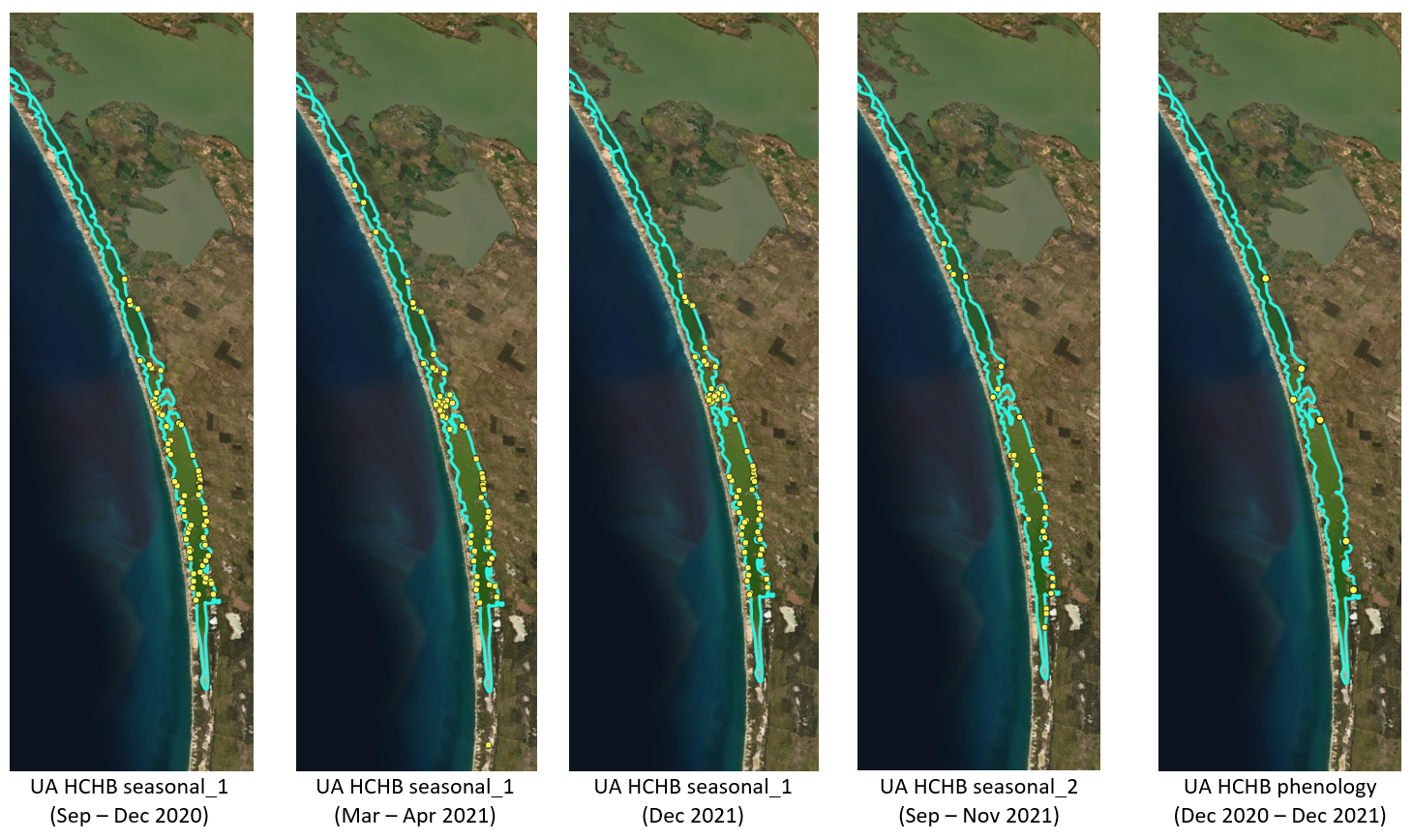
Figure 8.12: Ruppia sampling sites for the HCHB program. Agency/program code under each map corresponds to those listed in Table 8.4. Turquoise outline represents the model boundary.
8.1.4 Model application
This section describes both the Generation 0 model, which is the original model developed before HCHB, and the Generation 2.0 model, which was developed during HCHB.
8.1.4.1 Generation 0 model
The hydrodynamic-biogeochemical model TUFLOW-FV – AED was used to simulate hydrodynamic conditions (velocity, salinity, temperature and water level), water clarity (light and turbidity) and the potential for filamentous algae (nutrients and algae). Specifically, the HCHB V0.1 model was applied, configured using the specification of AED parameters (…). The Coorong has a long residence time and to account for the longer timescales of water and solute flux, multi-year simulations must be performed. The habitat suitability functions for each environmental variable of each Ruppia life-stage were determined based on literature review and expert judgement (Table 8.5 and Table 8.6), and used for the calculation of HSI for each life-stage (Equation (8.1) and Equation (8.2)). The HSI for each life-stage were integrated into an overall HSI for
- Completing the sexual reproduction annual cycle by going through seed germination in autumn, adult growth in winter and flowering and seed set in spring; or
- Completing the asexual reproduction annual cycle by going through turion sprouting in autumn, adult growth in winter and turion formation in spring. Specifically:
\[ \Phi^{HSI sexual}_{c} = \text{min}\left[\Phi^{HSI_{seed}}_{i},\Phi^{HSI_{adult}}_{i},\Phi^{HSI_{flower}}_{i} \right]_{c} \tag{8.5} \]
\[ \Phi^{HSI asexual}_{c} = \text{min}\left[\Phi^{HSI_{sprout}}_{i},\Phi^{HSI_{adult}}_{i},\Phi^{HSI_{turion}}_{i} \right]_{c} \tag{8.6} \]
| Life-stage, \(j\) | Seed germination/Turion sprouting | Adult growth | Flowering/Turion formation |
|---|---|---|---|
| Start date, \(t_{jstart}\) | Apr 1 | Jun 1 | Aug 1 |
| End date, \(t_{jend}\) | Jul 31 | Sep 30 | Dec 31 |
| Life stage |
f(S): Salinity (g/L) |
f(WL): Water depth (m) |
f(T): Temperature (°C) |
f(l): Light (%SI) |
f(FA): Algal biomass (g DW/m2) |
|---|---|---|---|---|---|
|
Seed germination (Apr 1 – Jul 30) |
<10 unsuitable 10-30 suboptimal 30-60 optimal 60-85 suboptimal >85 unsuitable |
Permanent dry: unsuitable <15 days wet (>95% of time): unsuitable 15-42 days wet (>95% of time): suboptimal* >42 days wet (>95% of time): optimal* Permanently wet: optimal |
<4 unsuitable 4-10 suboptimal 10-20 optimal 20-30 suboptimal >30 unsuitable |
- | - |
|
Turion sprouting (Apr 1 – Jul 30) |
<=0.1 unsuitable 0.1-20 suboptimal 20-75 optimal 75-130 suboptimal >130 unsuitable |
< 10 % of time wet: unsuitable >= 10 % of time wet: suitable |
<4 unsuitable 4-10 suboptimal 10-20 optimal 20-30 suboptimal >30 unsuitable |
<=7.5 unsuitable 7.5-24 suboptimal >=24 optimal |
- |
|
Adult plant growth (Jun 1 – Sep 30) |
<10 unsuitable 10-30 suboptimal 30-123 optimal 123-230 suboptimal >230 unsuitable |
< 10 % of time wet: unsuitable >= 10 % of time wet: suitable |
<4 unsuitable 4-10 suboptimal 10-20 optimal 20-30 suboptimal >30 unsuitable |
<=7.5 unsuitable 7.5-24 suboptimal >=24 optimal |
<=25 optimal 25-100 suboptimal >100 unsuitable |
|
Flowering and seed set (Aug 1 – Dec 31) |
<10 unsuitable 10-35 suboptimal 35-62 optimal 62-100 suboptimal >100 unsuitable |
<0.01 unsuitable 0.01-0.1 suboptimal 0.1-0.4 optimal 0.4-1 suboptimal >1 unsuitable |
<4 unsuitable 4-10 suboptimal 10-20 optimal 20-30 suboptimal >30 unsuitable |
- |
<=25 optimal 25-100 suboptimal >100 unsuitable |
|
Turion formation (Aug 1 – Dec 31) |
<70 unsuitable 70-124 suboptimal 124-160 optimal 160-230 suboptimal >230 unsuitable |
< 10 % of time wet: unsuitable >= 10 % of time wet: suitable |
<4 unsuitable 4-10 suboptimal 10-20 optimal 20-30 suboptimal >30 unsuitable |
- | - |
*Provided that the wet days are not followed by >8 dry
days (= unsuitable). Note: for Salinity,
Temperature, Light and Algal biomass, use 90-day rolling mean values for
the respective periods to interrogate the model outputs against these
thresholds
In these tests, the model was run from May 2013 to March 2019 using the base case condition. The outputs of the model are maps of habitat suitability of critical life stages (Figure 8.13, showing only the flowering stage in 2018), in response to light, depth, salinity and filamentous algae presence, which in the end results in a combined probability of sexual or asexual life-cycle completion (Figure 8.14, showing only the overall HSI for the completion of the sexual life cycle in 2018). The requirements for each life stage are quite different, and when each is superimposed together, the areas where life-cycle completion are limited to the margins of the main lagoons, and the shallow areas around the central region. From year to year, the area of good habitat changes, depending on that year’s eco-hydrodynamic regime.
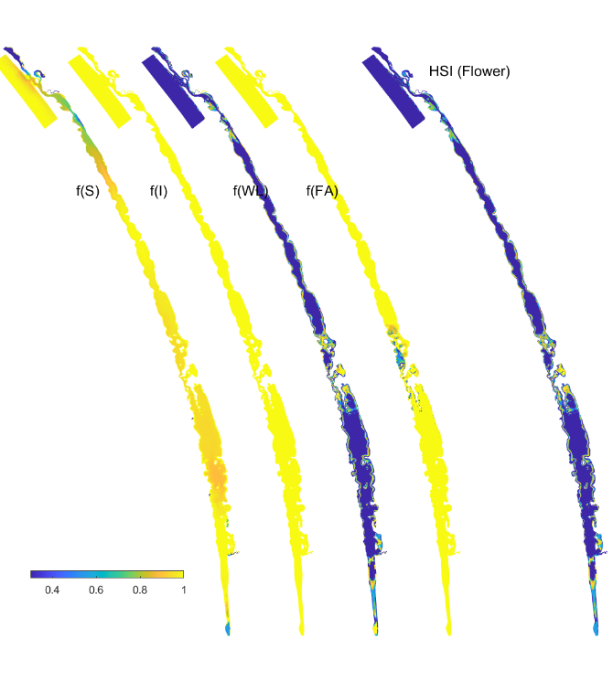
Figure 8.13: Habitat suitability (HSI) for the flowering plant phase of Ruppia tuberosa in the Coorong as a function of salinity f(S), light f(l), water level f(WL), and presence of filamentous algae f(FA) for the Base Case in 2018.An HSI of 0 (dark purple) represents unsuitable habitat conditions, while an HSI of 1 represents optimal conditions (yellow).
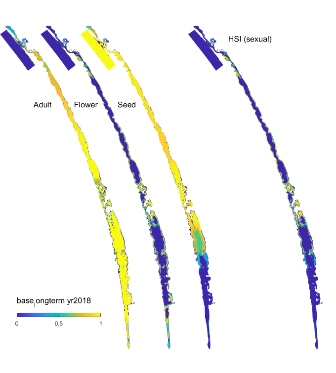
Figure 8.14: Overall HSI for the successful completion of the sexual life cycle of Ruppia tuberosa calculated by integrating the HSI results for adult plants, flowering and seedset, and seed germination in the Coorong, for the Base Case in 2018. An HSI of 0 (dark purple) represents unsuitable habitat conditions, while an HSI of 1 represents optimal conditions (yellow).
8.1.4.2 Generation 2.1 model
The hydrodynamic-biogeochemical model TUFLOW-FV – AED was used to simulate the hydrodynamic conditions (velocity, salinity, temperature and water level), water clarity (light and turbidity) and the potential for filamentous algae (nutrients and algae). Specifically, the HCHB Generation 2.1 model was applied, configured using the specification of AED parameters (…). The Coorong has a long residence time and to account for the longer timescales of water and solute flux, multi-year simulations must be performed. The habitat suitability functions for each environmental variable of each Ruppia life-stage were determined based on recent literature review, analyses of the HCHB survey data and expert judgement (Table 8.7, Table 8.8, Appendix C), and used for the calculation of HSI for each life-stage (Equation (8.1) and Equation (8.2)). The HSI for each life-stage were integrated into
An overall HSI sexual, representing the integrated habitat suitability for Ruppia to complete its annual life cycle by reproducing sexually, i.e., flowering, which includes i) emerging in autumn, either from germination from seed or sprouting from viable turions that survived the summer; ii) vegetative growth to adult plants in winter; and iii) successful flowering and producing seed in spring; or
An overall HSI asexual, representing the integrated habitat suitability for Ruppia to complete its annual life cycle by reproducing asexually, i.e., forming turions, which includes i) emerging in autumn, either from germination from seed or sprouting from viable turions that survived the summer; ii) vegetative growth to adult plants in winter; and iii) formation of turions in spring. Specifically:
\[ \Phi^{HSI sexual}_{c} = \text{min}\left[\text{max}\left[\Phi^{HSI_{seed}}_{i},\text{min}\left[\Phi^{HSI_{viability}}_{i},\Phi^{HSI_{sprout}}_{i}\right]\right],\Phi^{HSI_{adult}}_{i},\Phi^{HSI_{flower}}_{i}\right]_{c} \tag{8.7} \]
\[ \Phi^{HSI asexual}_{c} = \text{min}\left[\text{max}\left[\Phi^{HSI_{seed}}_{i},\text{min}\left[\Phi^{HSI_{viability}}_{i},\Phi^{HSI_{sprout}}_{i}\right]\right],\Phi^{HSI_{adult}}_{i},\Phi^{HSI_{turion}}_{i}\right]_{c} \tag{8.8} \]
This new HSI integration approach differs from the Generation 0
model in two ways:
A new function, turion viability was added to the model for the summer dormancy period and integrated in the HSI calculation before turion sprouting to exclude areas where salinity levels were sufficiently high to cause ion toxicity in turions during summer. Kim et al. (2013) showed that after exposure to high salinities for 60 days, most turions lost viability and failed to sprout after being transferred back to fresher conditions. In comparison, seed viability was not negatively affected by high salinities.
For the beginning of Ruppia’s life cycle in autumn, the probability of both seed germination and turion sprouting are included in both sexual and asexual pathways, whereas in the previous version, seed germination was exclusive to the calculation of HSI sexual and turion sprouting exclusive to HSI asexual. The rationale behind this change is because Ruppia individuals that ended up flowering may not necessarily have started from seed germination but could be from turion sprouting. Likewise, Ruppia individuals that formed turions in the end could have started from seed germination.
| Life-stage, \(j\) | Turion viability | Seed germination/Turion sprouting | Adult growth | Flowering/Turion formation |
|---|---|---|---|---|
| Start date, \(t_{jstart}\) | Jan 1 | Apr 1 | Jun 1 | Sep 1 |
| End date, \(t_{jend}\) | Mar 31 | Jun 30 | Sep 30 | Dec 31 |
| Life stage |
f(S): Salinity (g/L) |
f(WL): Water depth (m) |
f(T): Temperature (°C) |
f(l): Light (%SI) |
f(FA): Algal biomass (g DW/m2) |
|---|---|---|---|---|---|
|
Turion viability (Jan 1 - Mar 31) |
<135 optimal 135–165 suboptimal >=165 unsuitable |
- | - | - | - |
|
Seed germination (Apr 1 – Jul 30) |
<=0.1 unsuitable 0.1-40 optimal 40-85 suboptimal >85 unsuitable |
Permanent dry: unsuitable <15 days wet (>95% of time): unsuitable 15-42 days wet (>95% of time): suboptimal* >42 days wet (>95% of time): optimal* Permanently wet: optimal |
<4 unsuitable 4-10 suboptimal 10-23 optimal 23-30 suboptimal >30 unsuitable |
- | - |
|
Turion sprouting (Apr 1 – Jul 30) |
<=0.1 unsuitable 0.1-20 suboptimal 20-75 optimal 75-125 suboptimal >125 unsuitable |
< 10 % of time wet: unsuitable >= 10 % of time wet: suitable |
<4 unsuitable 4-10 suboptimal 10-23 optimal 23-30 suboptimal >30 unsuitable |
<=5 unsuitable 5-36 suboptimal >=36 optimal |
- |
|
Adult plant growth (Jun 1 – Sep 30) |
<10 unsuitable 10-19 suboptimal 19-124 optimal 124-230 suboptimal >230 unsuitable |
< 10 % of time wet: unsuitable >= 10 % of time wet: suitable |
<4 unsuitable 4-10 suboptimal 10-23 optimal 23-30 suboptimal >30 unsuitable |
<=5 unsuitable 5-36 suboptimal >=36 optimal |
<=100 optimal 100-368 suboptimal >368 unsuitable |
|
Flowering and seed set (Aug 1 – Dec 31) |
<12 unsuitable 12-47 suboptimal 47-62 optimal 62-100 suboptimal >100 unsuitable |
<0.1 unsuitable 0.1-0.4 optimal 0.4-0.9 suboptimal >0.9 unsuitable |
<4 unsuitable 4-10 suboptimal 10-23 optimal 23-30 suboptimal >30 unsuitable |
<=5 unsuitable 5-36 suboptimal >=36 optimal |
<=100 optimal 100-184 suboptimal >184 unsuitable |
|
Turion formation (Aug 1 – Dec 31) |
<40 unsuitable 40-70 suboptimal 70-160 optimal 160-230 suboptimal >230 unsuitable |
< 10 % of time wet: unsuitable >= 10 % of time wet: suitable |
<4 unsuitable 4-10 suboptimal 10-23 optimal 23-30 suboptimal >30 unsuitable |
<=5 unsuitable 5-36 suboptimal >=36 optimal |
- |
*Provided that the wet days are not followed by >8 dry days (= unsuitable).
In these tests, the model was run from July 2017 to Nov 2022 using
the base case condition. The outputs of the model are maps of habitat
suitability of critical life stages (Figure 8.15),
showing only the flowering stage in 2020), in response to light, depth,
salinity, temperature and filamentous algae presence, which in the end
results in a combined probability of sexual or asexual life-cycle
completion (Figure 8.16, showing only the overall
HSI for the completion of the sexual life cycle in 2020). The
requirements for each life stage are quite different, and when each is
superimposed together, the areas where life-cycle completion are limited
to the margins of the main lagoons, and the shallow areas around the
central region. From year to year, the area of good habitat changes,
depending on that year’s eco-hydrodynamic regime.
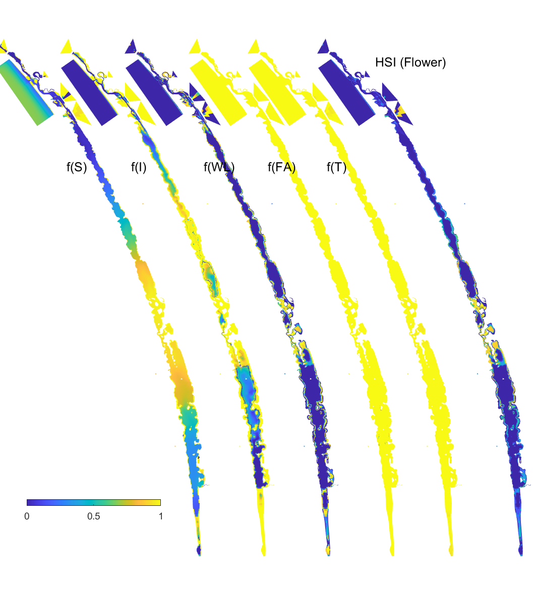
Figure 8.15: Habitat suitability (HSI) for the flowering plant phase of Ruppia tuberosa in the Coorong as a function of salinity f(S), light f(l), water level f(WL), temperature f(T) and presence of filamentous algae f(FA) for the base case in 2020. An HSI of 0 (dark purple) represents unsuitable habitat conditions, while an HSI of 1 represents optimal conditions (yellow).
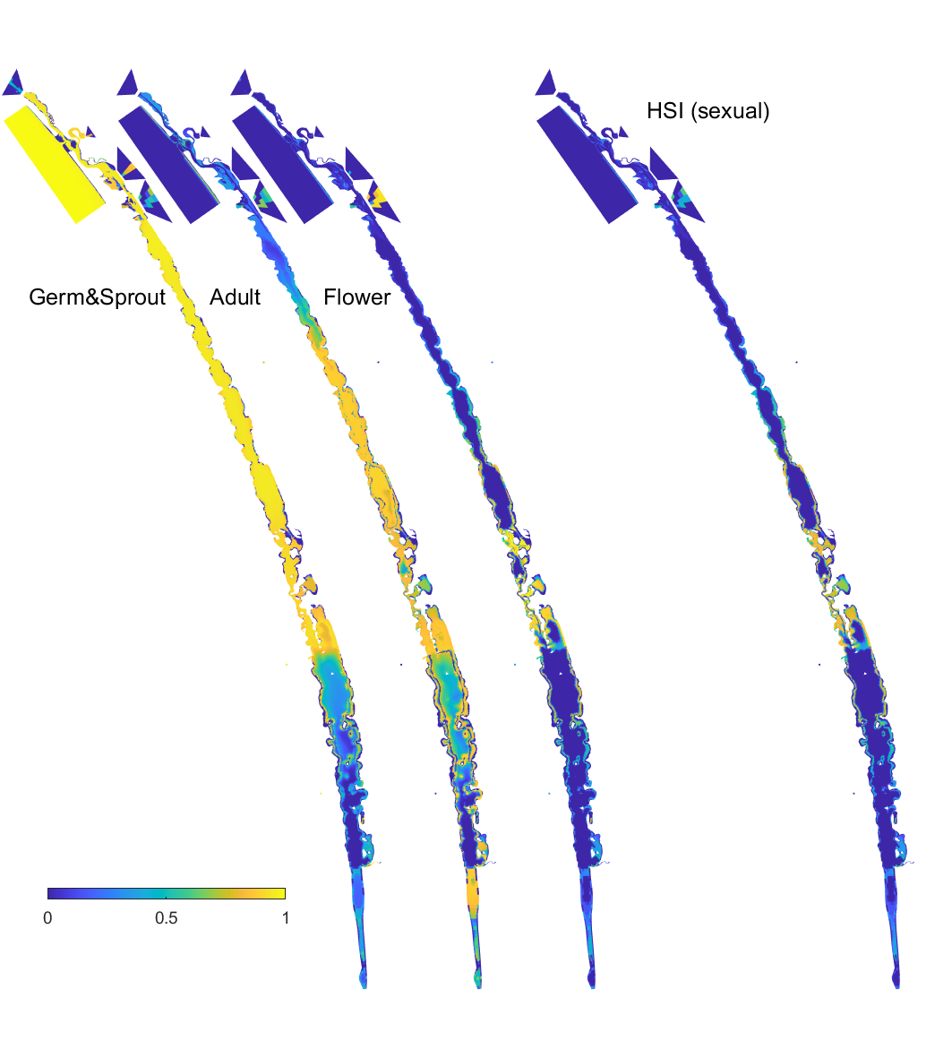
Figure 8.16: Overall HSI for the successful completion of the sexual life cycle calculated by integrating the HSI results for seed germination, turion viability and turion sprouting, adult plants, and flowering and seed set in the Coorong, for the Base Case in 2020. An HSI of 0 (dark purple) represents unsuitable habitat conditions, while an HSI of 1 represents optimal conditions (yellow).
8.1.5 Model results and assessment
To assess the accuracy of model predictions, the habitat suitability
maps produced above were compared with Ruppia field survey results for
both distribution and abundance, including several types of plant
materials (e.g., shoot, seed, turion) which were used to validate HSI of
different life-stages. In addition to a visual assessment, regression
analyses were conducted in R studio between HSI values and Ruppia
abundance for each life-stage over relevant periods. In general, this
was done by overlaying Ruppia spatial data on HSI maps, creating a
buffer around each sampling site, averaging HSI values in each model
cell that fall within this buffer, and comparing with Ruppia
abundance.
The specific validation approach has evolved as the
project progresses with more data becoming available, model updates
implemented, and more insights revealed. For example, the strategies for
pairing specific plant material recorded in the field with HSI output of
a particular life-stage (e.g. seed abundance in Mar vs. HSI flowering in
Sep the previous year) and its appropriate timing has initially been
explored extensively. Table 8.9 summarises the
various major validation versions, including their data source, model
version and methodology. Details of methods and results of the latest
version ‘HCHB_Gen 2.1,’ in which the Gen 2.1 model were implemented are
described below. Details of assessments of previous versions and
evolution of validation approaches are included in Appendix C.
| Validation version | Field data | Hydro- dynamic model | Environmental thresholds | Life-stage time windows | Life-stage integration | Model output timeframe | Buffer radius (m) | HSI averaging within buffer |
|---|---|---|---|---|---|---|---|---|
|
Historical (Appendix C) |
Historical (2016 - 2019) |
Gen 0 |
Gen 0 (Table 8.6) |
Gen 0 (Table 8.5) |
Gen 0 (Eq.8.5 - 8.6) |
default | 600 | arithmetic |
|
HCHB_v1 (Appendix C) |
HCHB (Sep 2020 – Apr 2021) |
Gen 0 |
Gen 0 (Table 8.6) |
Gen 0 (Table 8.5) |
Gen 0 (Eq.8.5 - 8.6) |
default | 600 or 100 | arithmetic |
|
HCHB_v2 (Appendix C) |
HCHB (Sep 2020 – Apr 2021) |
Gen 0 |
Gen 0 (Table 8.6) |
Gen 0 (Table 8.5) |
Gen 2.0 (Eq.8.7 - 8.8)* |
tailored | 100 |
spatial (area-weighted) |
|
HCHB_Gen 2.0 (Appendix C) |
HCHB (Sep 2020 – Dec 2021); MDBA (2018 - 2019) |
Gen 2.0 |
Gen 2.0 (Table 8.8) |
Gen 2.0 (Table 8.7) |
Gen 2.0 (Eq.8.7 - 8.8) |
tailored | 100 |
spatial (area-weighted) |
| HCHB_Gen 2.1 |
HCHB (Sep 2020 – Dec 2021) |
Gen 2.1 |
Gen 2.0 (Table 8.8) |
Gen 2.0 (Table 8.7) |
Gen 2.0 (Eq.8.7 - 8.8) |
tailored | 100 |
spatial (area-weighted) |
*Excludes turion viability function
HCHB Gen 2.1 validation
Ruppia survey data and associated model output used for the Gen 2.1
model assessment as well as model error metrics are summarised in Table
8.10, and results described in following subsections.
In addition to Spearman’s rank correlation coefficients (rs), two
additional error metrics were calculated:
- overall goodness-of-fit (fit), expressed as % of all survey sites, was calculated by
\[ fit = \frac{\text{number of instances of True Positive + number of instances of True Negative}}{\text{total number of instances}}*100 \] Where True Positive (TP) refers to sites where Ruppia density is greater than the median density of all sites surveyed in that season and modelled HSI > 0.5, while True Negative (TN) refers to sites where Ruppia density is lower than the median density and modelled HSI ≤ 0.5.
- score, calculated by
\[ score = \frac{\text{proportion of sites containing major biomass within suitable habitat}}{\text{proportion of survey sites containing suitable habitat}} \] Where sites containing major biomass refers to sites where Ruppia density is greater than the median density of all sites surveyed in that season; and suitable habitat refers to HSI > 0.5. The model prediction is informative if score > 1, whereas if score ≤ 1 Ruppia is randomly distributed.
Note that while Gen 2.1 hydrodynamic model was extended to 2022 with a refined mesh, Ruppia model performance was assessed up to 2021 only since field data were unavailable for 2022.
Overall, Gen 2.1 model produced similar Ruppia HSI predictions to Gen 2.0, with some improvements in error metrics for some life-stages in 2021 (Table8.10). The additional two error metrics, fit and score, introduced in the Gen 2.1 testing suggested that the model can predict True Positive and True Negative reasonably well with an average overall goodness-of-fit of 65% for all life-stages across both years, and that model predictions were informative (score > 1) for all life-stages except for shoot and flower in 2021.
| Survey data | Survey period | Model output | Model integration period |
rs (Whole lagoon) |
rs (South lagoon) |
fit (%, Whole lagoon) |
fit (%, South lagoon) |
score (Whole lagoon) |
score (South lagoon) |
|---|---|---|---|---|---|---|---|---|---|
| Shoot count (HCHB) | 9-12/2020 | HSI seed germination + turion viability + turion sprouting + adult growth | 1-9/2020 | 0.53 | 0.40 | 68 | 69 | 1.37 | 1.39 |
| Flower count (HCHB) | 9-12/2020 | HSI sexual | 1-10/2020 | 0.56 | 0.38 | 80 | 81 | 2.48 | 2.95 |
| Turion count (HCHB) | 9-12/2020 | HSI asexual | 1-10/2020 | 0.31 | 0.40 | 61 | 69 | 1.30 | 1.40 |
| Turion count (HCHB) | 3-4/2021 | HSI asexual | 1-10/2020 | 0.41 | 0.37 | 58 | 57 | 1.24 | 1.20 |
| Seed count (HCHB) | 3-4/2021 | HSI sexual | 1-12/2020 | 0.37 | 0.45 | 66 | 66 | 1.43 | 1.58 |
| Shoot count (HCHB) | 12/2021 | HSI seed germination + turion viability + turion sprouting + adult growth | 1-9/2021 | 0.22 | 0.34 | 48 | 42 | 0.94 | 0.85 |
| Flower count (HCHB) | 12/2021 | HSI sexual | 1-12/2021 | -0.13 | -0.11 | 72 | 76 | 0.00 | 0.00 |
| Seed count (HCHB) | 12/2021 | HSI sexual | 1-12/2021 | 0.20 | 0.11 | 74 | 77 | 1.24 | 0.89 |
| Turion count (HCHB) | 12/2021 | HSI asexual | 1-12/2021 | 0.57 | 0.51 | 57 | 49 | 1.62 | 1.01 |
i. Field shoot count Sep 2020 (obs) vs. HSI seed germination + turion viability + turion sprouting + adult growth Sep 2020 (model)
Average number of seagrass shoots per square meter recorded in Sep - Dec 2020 (reproductive period) were compared with combined HSI for seed germination, turion sprouting and adult growth up to end of Sep in the same year (Figure 8.17 and 8.18). The overall distribution of shoots was consistent with model prediction. Seagrass density around the middle lagoon and north lagoon were higher, where HSI predictions were highest.
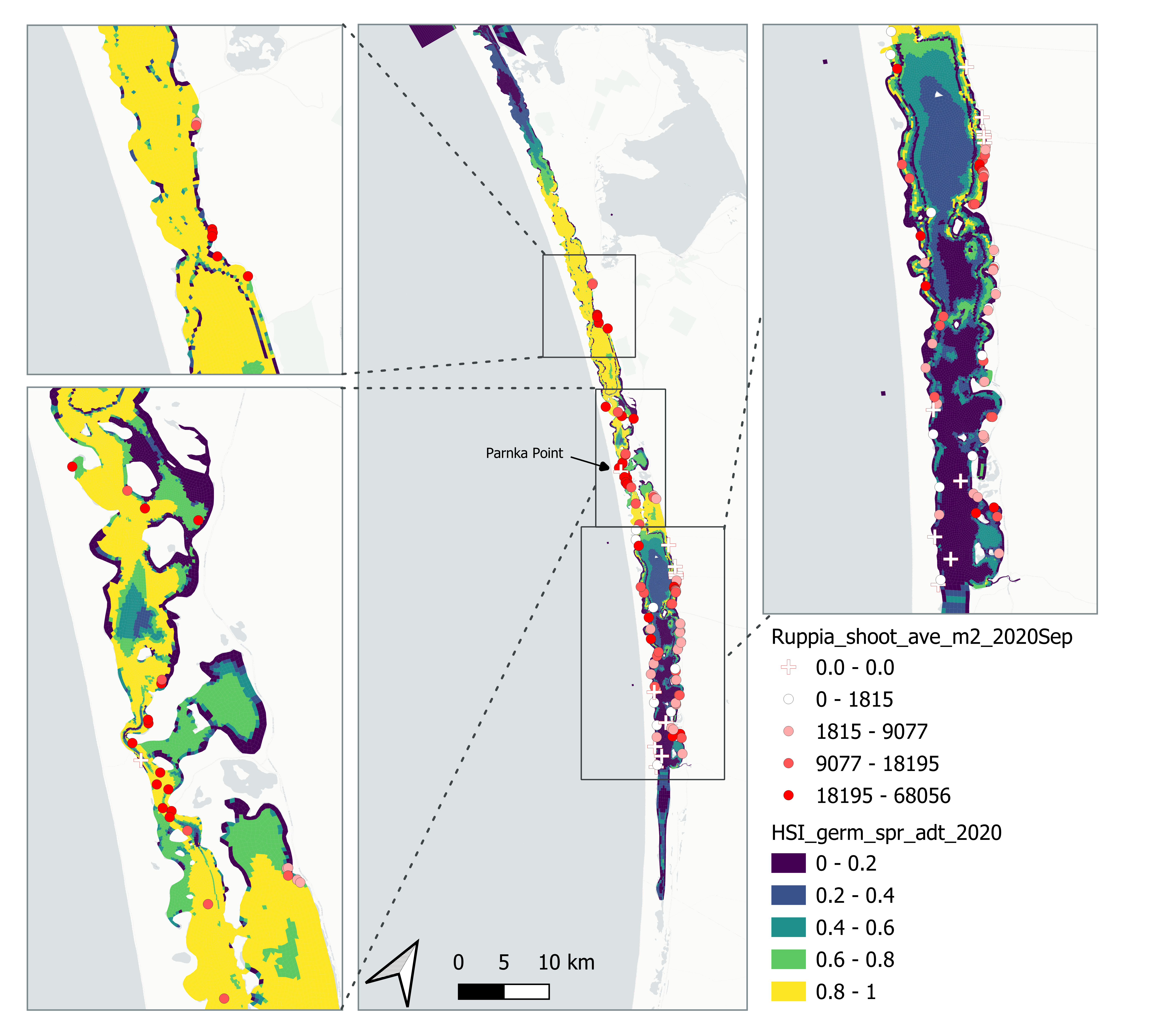
Figure 8.17: Average seagrass shoot count per square meter in Sep – Dec 2020 (circles) overlaid on HSI model output for germination, sprouting and adult growth integrated over Jan - Sep 2020. An HSI of 0 (dark purple) represents unsuitable habitat conditions, while an HSI of 1 represents optimal conditions (yellow).
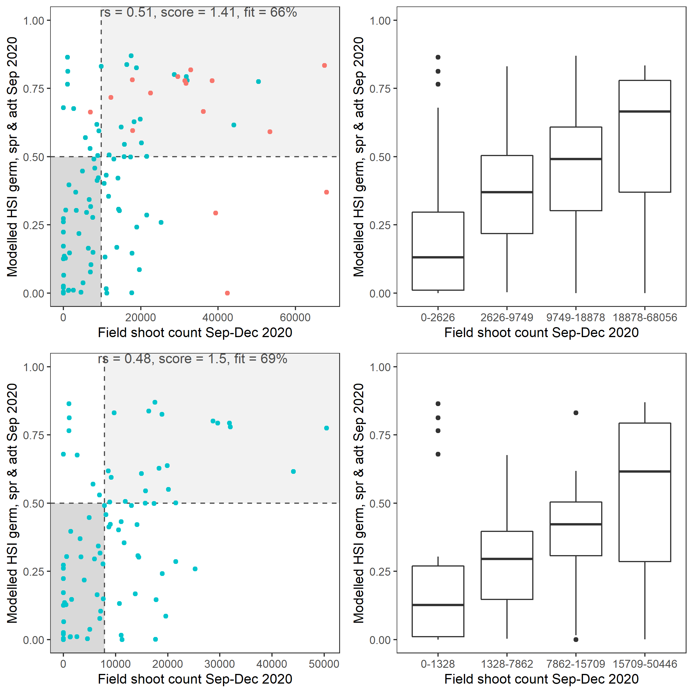
Figure 8.18: Scatter plot and boxplot of average seagrass shoot count per square meter in Sep – Dec 2020 versus HSI model output for germination, sprouting and adult growth integrated over Jan - Sep 2020. Top panel: the entire lagoon (red: north, blue: south), bottom panel: south lagoon. An HSI of 0 represents unsuitable habitat conditions, while an HSI of 1 represents optimal conditions. Vertical dashed line: median count; horizontal dashed line: HSI = 0.5, above which the habitat is classified as ‘preferred habitat’; points within light shaded area: True Positive; points within dark shaded area: True Negative.
ii. Field flower count Sep 2020 (obs) vs. HSI sexual Oct 2020 (model)
Average number of Ruppia flower per square meter recorded in Sep - Dec 2020 (reproductive period) were compared with overall HSI for sexual reproduction up to end of Oct in the same year (Figure 8.19 and 8.20). The overall distribution of flowers generally aligned with model prediction where the highest density of flowers occurred in suitable habitat (HSI > 0.5).
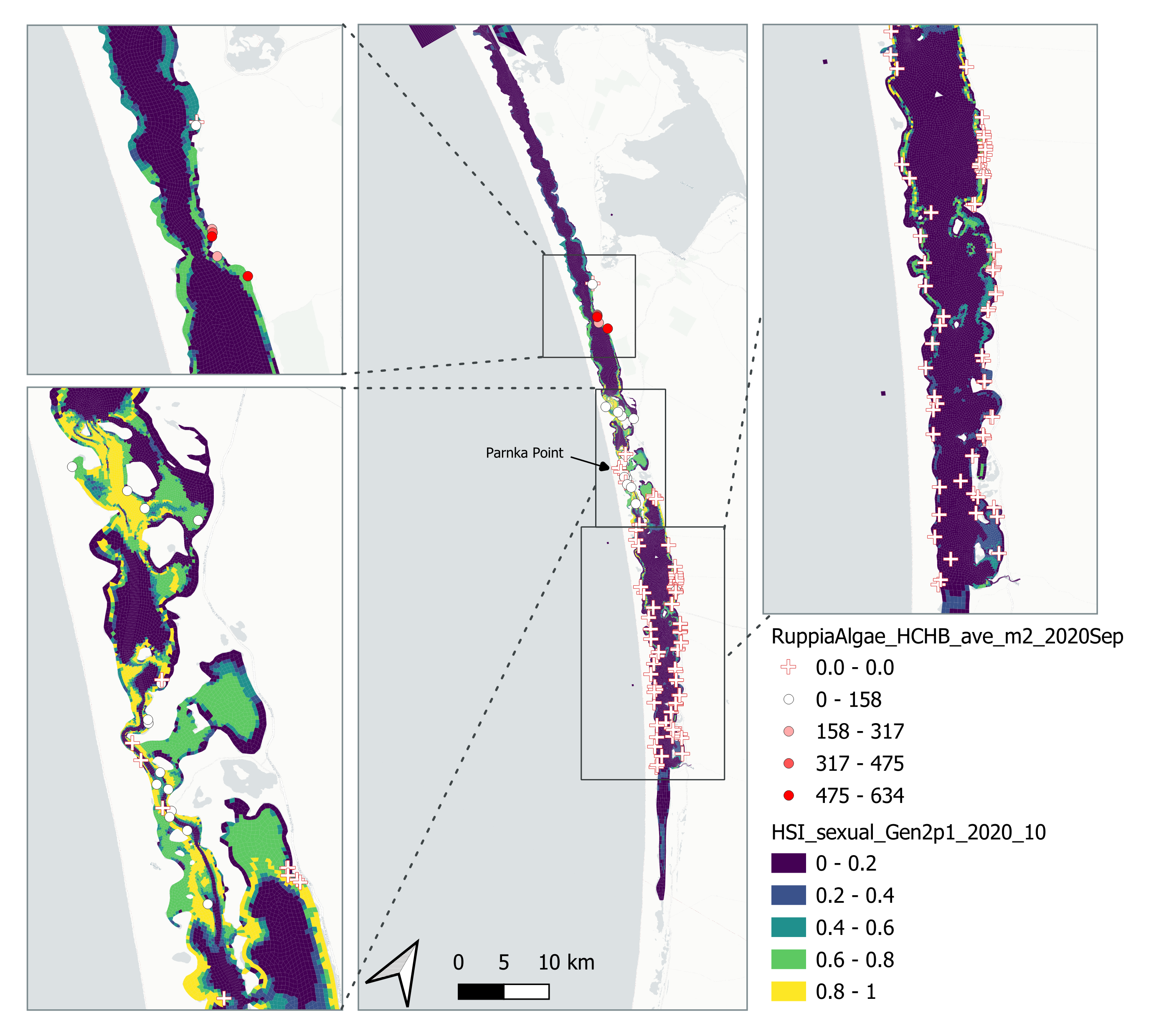
Figure 8.19: Average Ruppia flower count per square meter in Sep – Dec 2020 (circles) overlaid on HSI model output for overall sexual reproduction integrated over Jan – Oct 2020. An HSI of 0 (dark purple) represents unsuitable habitat conditions, while an HSI of 1 represents optimal conditions (yellow).
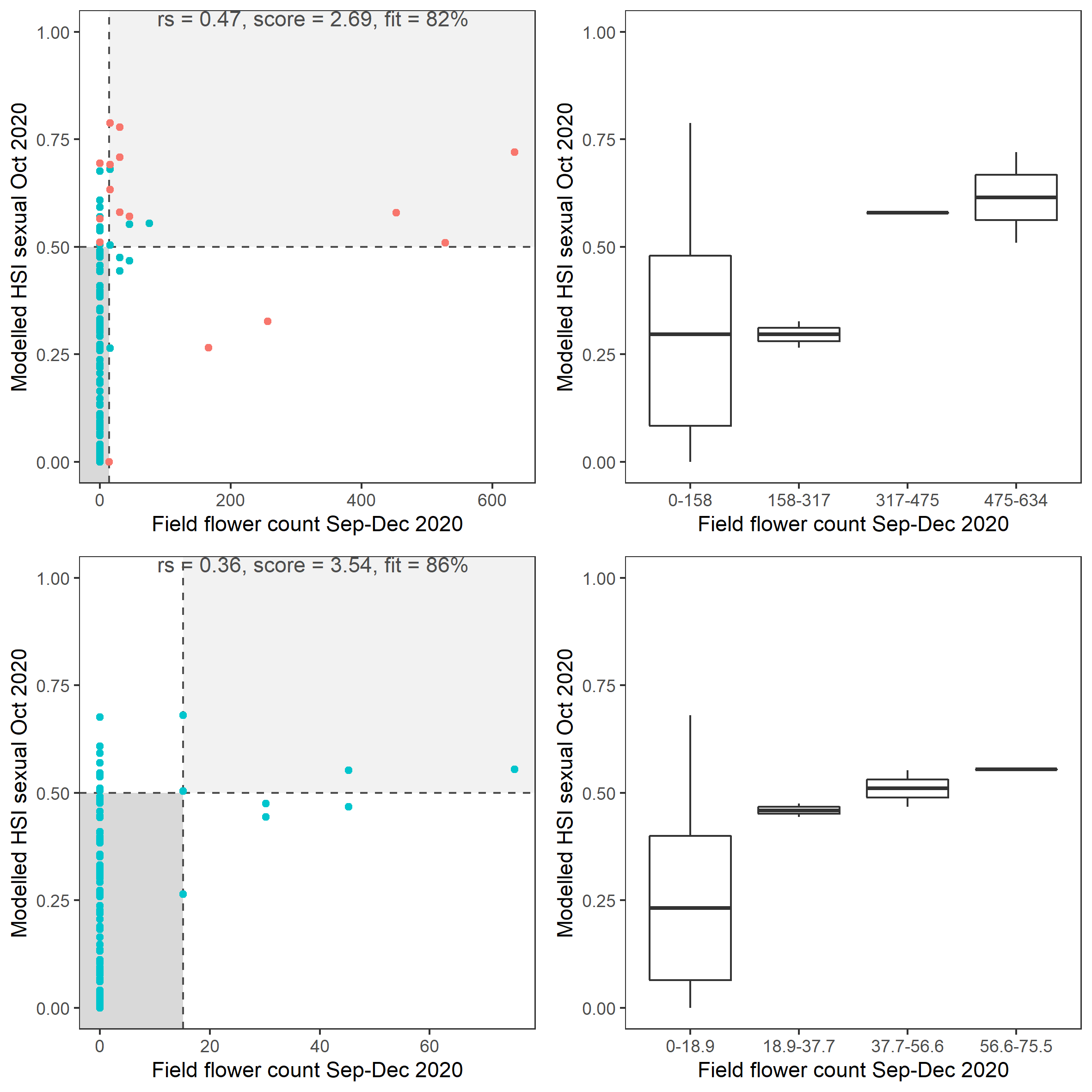
Figure 8.20: Scatter plot and boxplot of average Ruppia flower count per square meter in Sep – Dec 2020 versus HSI model output for overall sexual reproduction integrated over Jan - Oct 2020. Top panel: the entire lagoon (red: north, blue: south), bottom panel: south lagoon. An HSI of 0 represents unsuitable habitat conditions, while an HSI of 1 represents optimal conditions.Vertical dashed line: median count; horizontal dashed line: HSI = 0.5, above which the habitat is classified as ‘preferred habitat’; points within light shaded area: True Positive; points within dark shaded area: True Negative.
iii. Field seed count Mar 2021 (obs) vs. HSI sexual Dec 2020 (model)
Average number of Ruppia tuberosa seed per square meter recorded in Mar - Apr 2021 (aestivation period) were compared with overall HSI for sexual reproduction in 2020 (Figure 8.21 and 8.22). It’s important to note that seeds have the potential to disperse with water current/wind therefore its distribution and abundance may be less predictable than other plant materials.
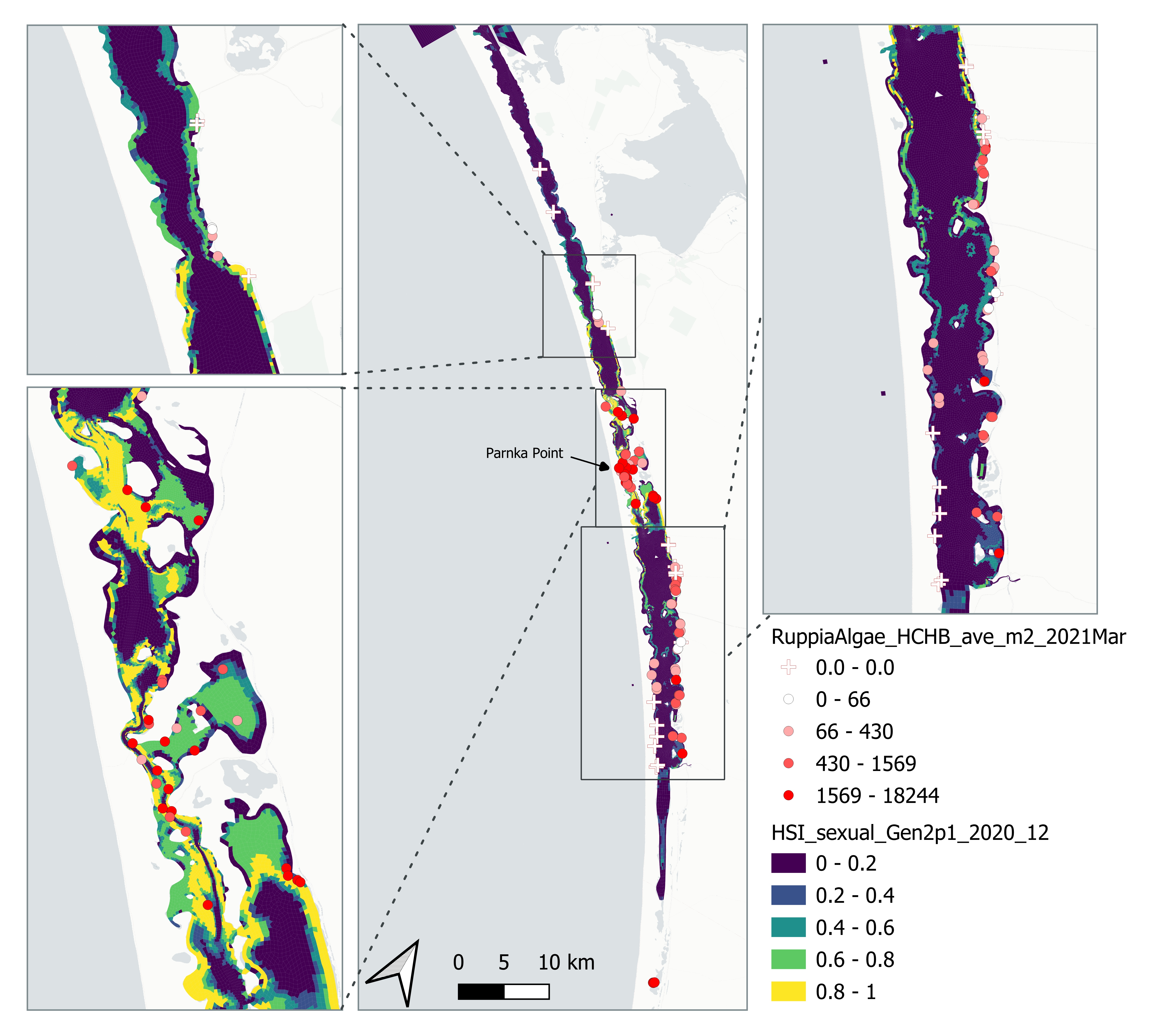
Figure 8.21: Average Ruppia tuberosa seed count per square meter in Mar – Apr 2021 (circles) overlaid on HSI model output for overall sexual reproduction integrated over Jan – Dec 2020. An HSI of 0 (dark purple) represents unsuitable habitat conditions, while an HSI of 1 represents optimal conditions (yellow).
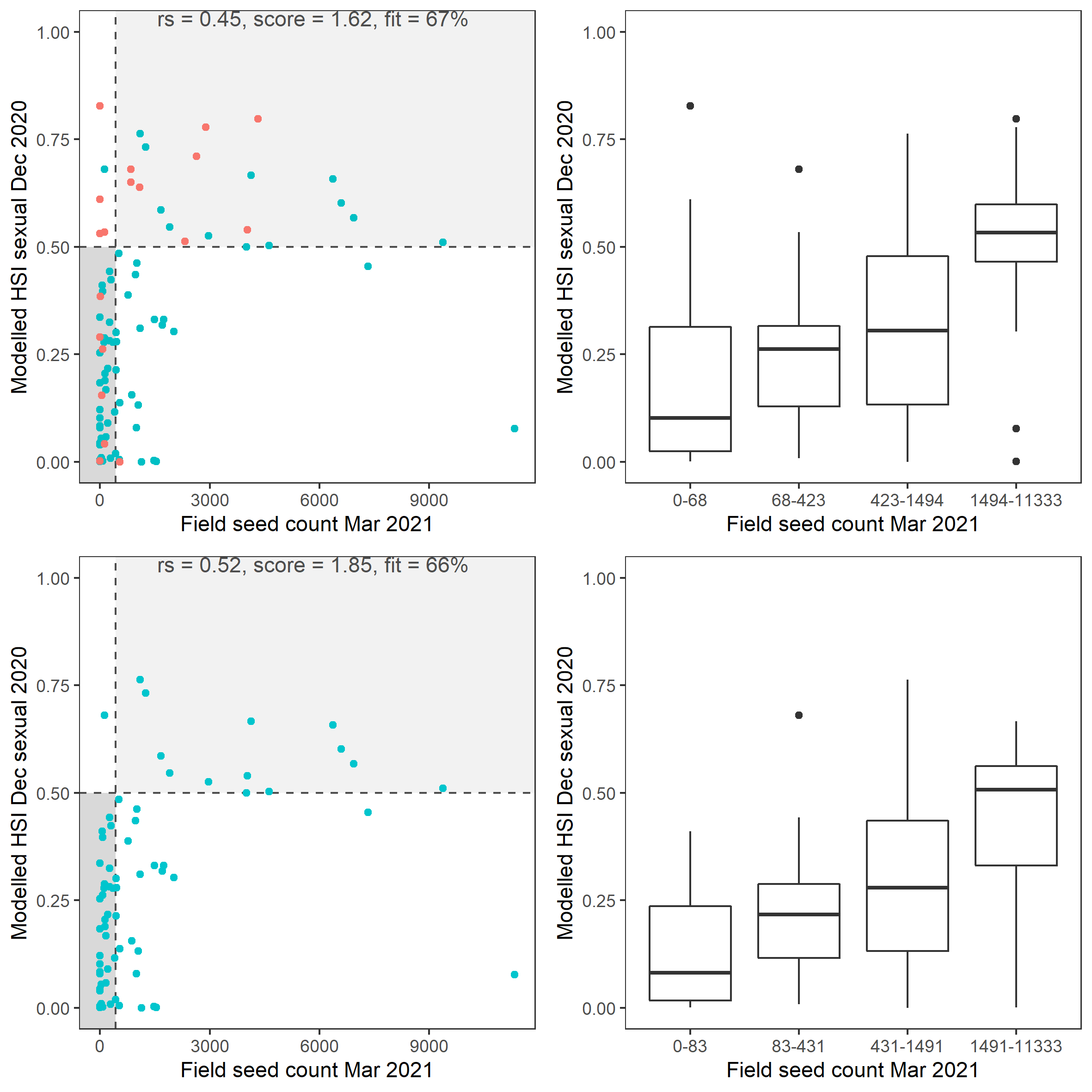
Figure 8.22: Scatter plot and boxplot of average Ruppia tuberosa seed count per square meter in Mar – Apr 2021 versus HSI model output for overall sexual reproduction integrated over Jan - Dec 2020. Top panel: the entire lagoon (red: north, blue: south), bottom panel: south lagoon. An HSI of 0 represents unsuitable habitat conditions, while an HSI of 1 represents optimal conditions. Vertical dashed line: median count; horizontal dashed line: HSI = 0.5, above which the habitat is classified as ‘preferred habitat’; points within light shaded area: True Positive; points within dark shaded area: True Negative.
iv. Field turion count Sep 2020 (obs) vs. HSI asexual Oct 2020 (model)
Average number of Ruppia turion (type I and II) per square meter recorded in Sep - Dec 2020 (reproductive period) were compared with overall HSI for asexual reproduction up to end of Oct in the same year (Figure 8.23 and 8.24). The overall distribution of turions agreed with model prediction although there were some misalignment in the North lagoon.
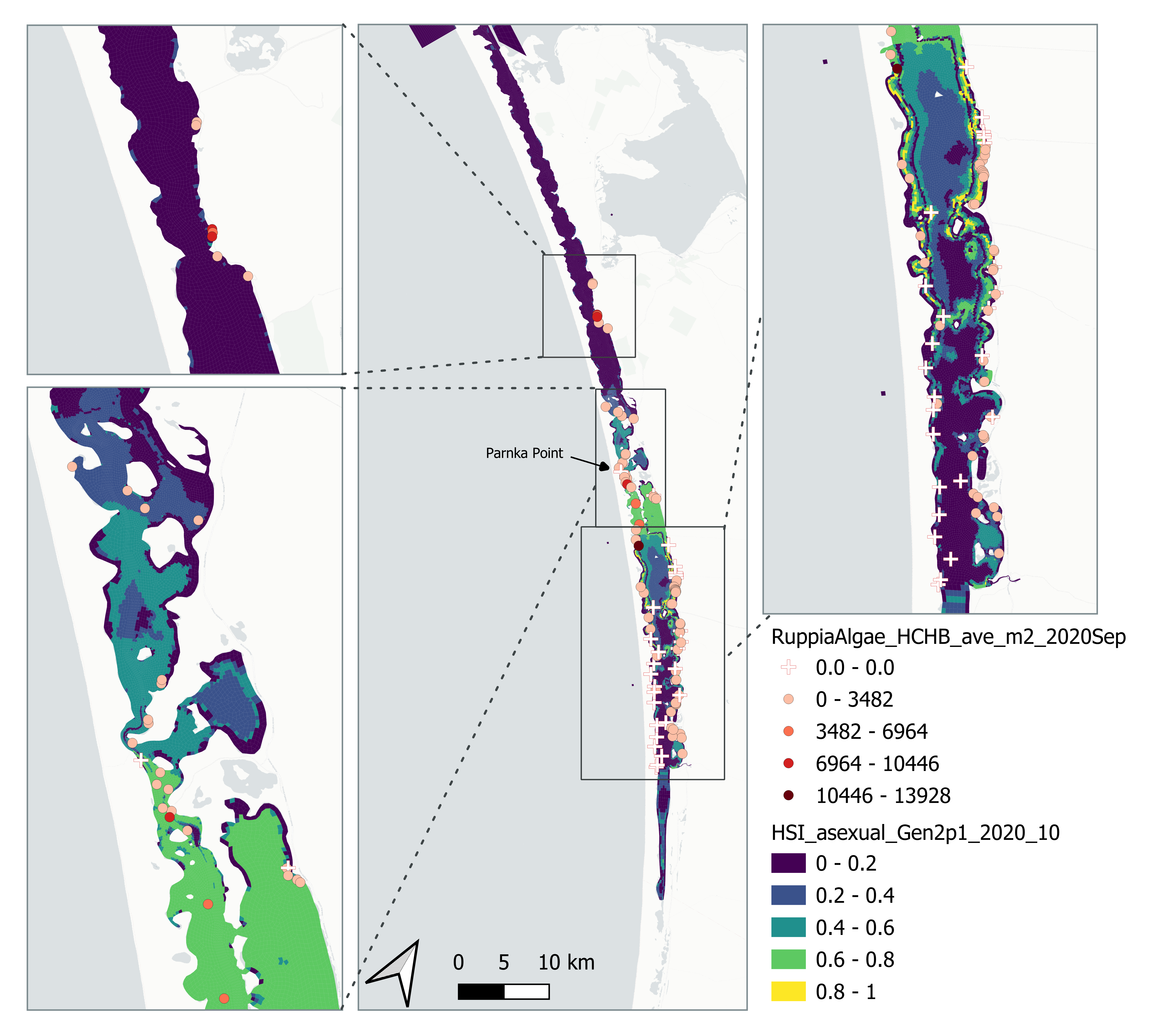
Figure 8.23: Average Ruppia turion count per square meter in Sep – Dec 2020 (circles) overlaid on HSI model output for overall asexual reproduction integrated over Jan – Oct 2020. An HSI of 0 (dark purple) represents unsuitable habitat conditions, while an HSI of 1 represents optimal conditions (yellow).
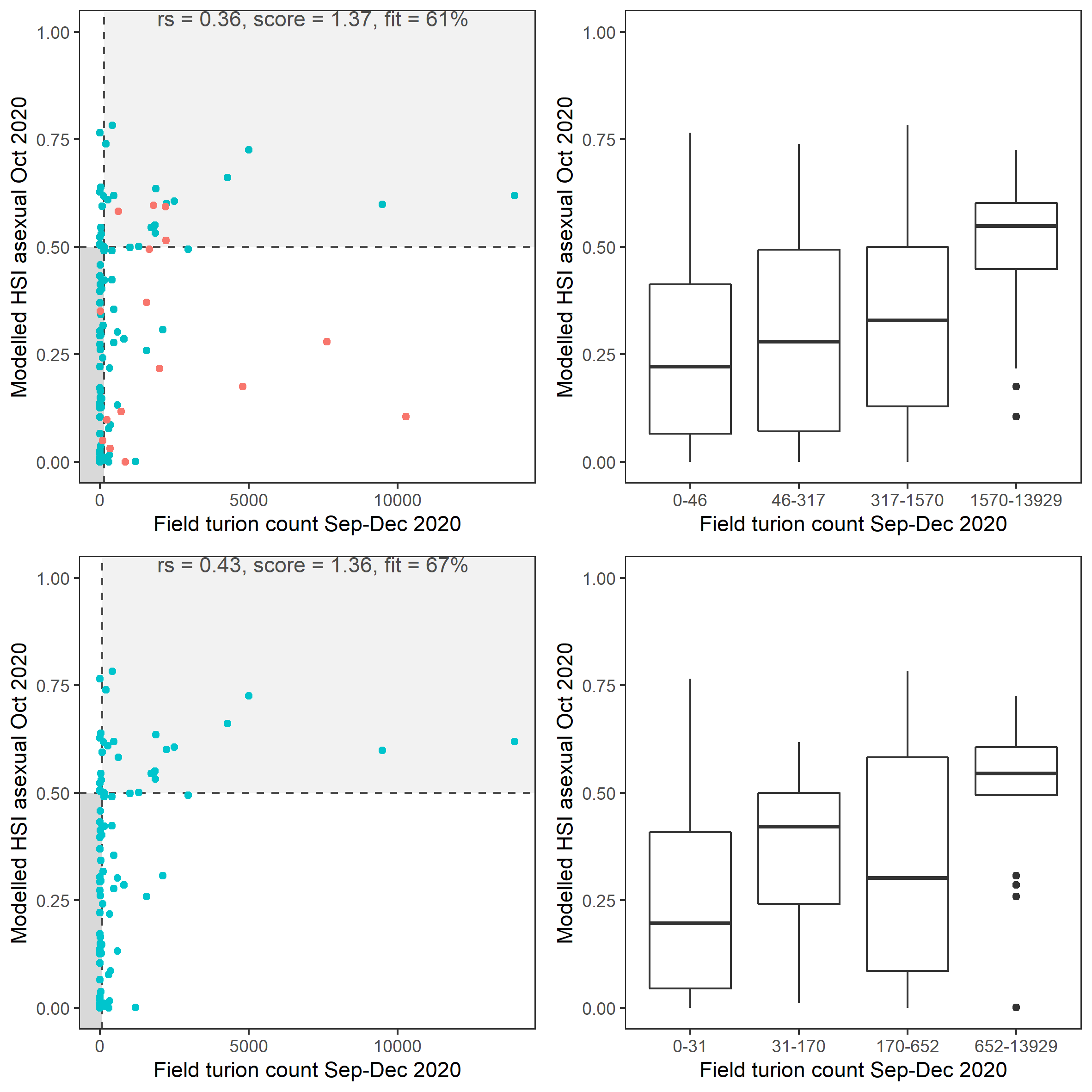
Figure 8.24: Scatter plot and boxplot of average Ruppia turion count per square meter in Sep – Dec 2020 versus HSI model output for overall asexual reproduction integrated over Jan - Oct 2020. Top panel: the entire lagoon (red: north, blue: south), bottom panel: south lagoon. An HSI of 0 represents unsuitable habitat conditions, while an HSI of 1 represents optimal conditions. Vertical dashed line: median count; horizontal dashed line: HSI = 0.5, above which the habitat is classified as ‘preferred habitat’; points within light shaded area: True Positive; points within dark shaded area: True Negative.
v. Field shoot count Dec 2021 (obs) vs. HSI seed germination + turion viability + turion sprouting + adult growth Sep 2021 (model)
Average number of seagrass shoots per square meter recorded in Dec 2021 (reproductive period) were compared with combined HSI for seed germination, turion sprouting and adult growth up to end of Sep in the same year (Figure 8.25 and 8.26). The validation scores of 2021 were lower than that of 2020, possibly due to the environmental conditions experienced in winter-spring 2021 (including unusually cool and wet conditions), which may have caused a delay in the Ruppia life cycle (Waycott 2022, pers. comm.).
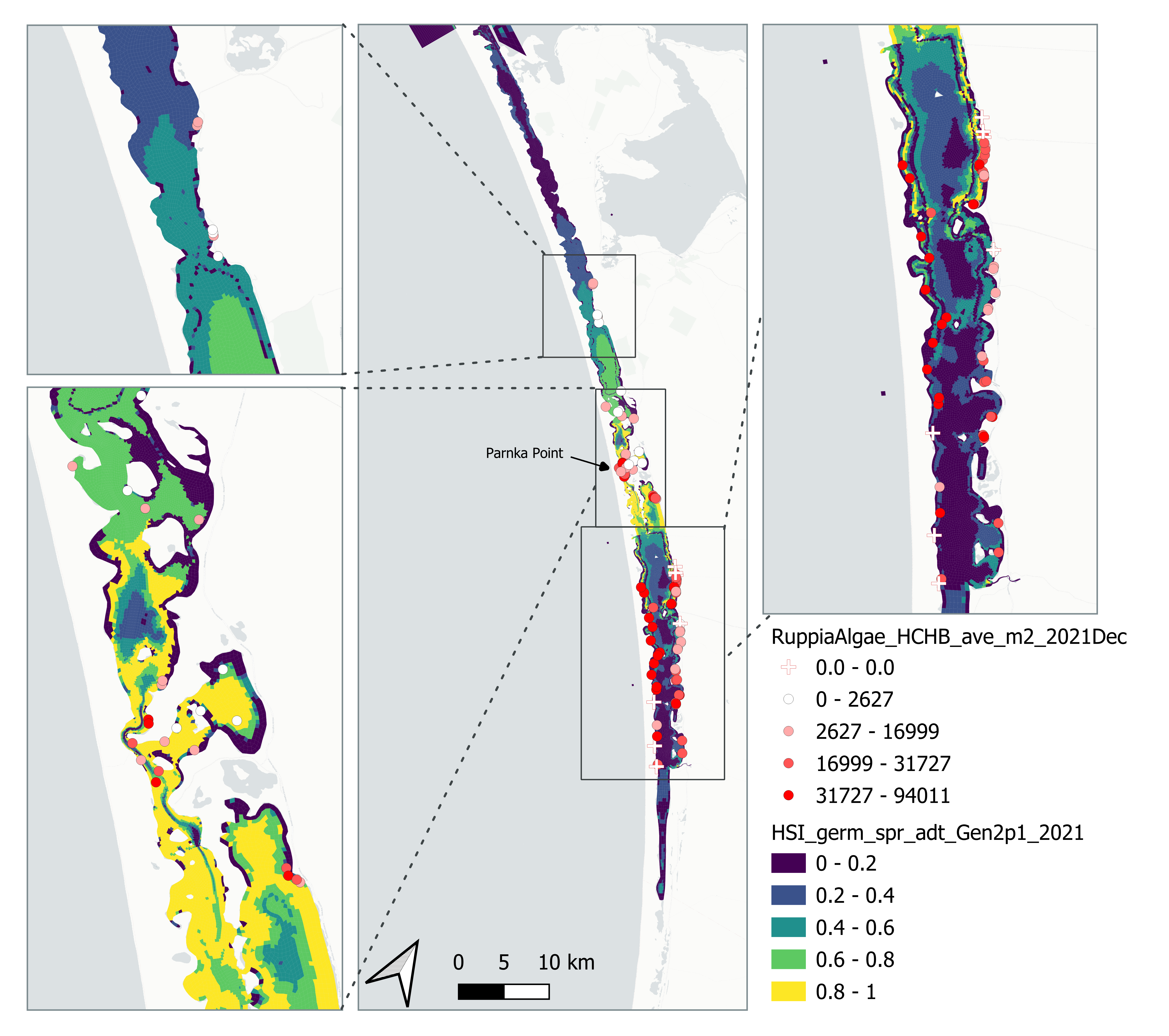
Figure 8.25: Average seagrass shoot count per square meter in Dec 2021 (circles) overlaid on HSI model output for germination, sprouting and adult growth integrated over Jan - Sep 2021. An HSI of 0 (dark purple) represents unsuitable habitat conditions, while an HSI of 1 represents optimal conditions (yellow).
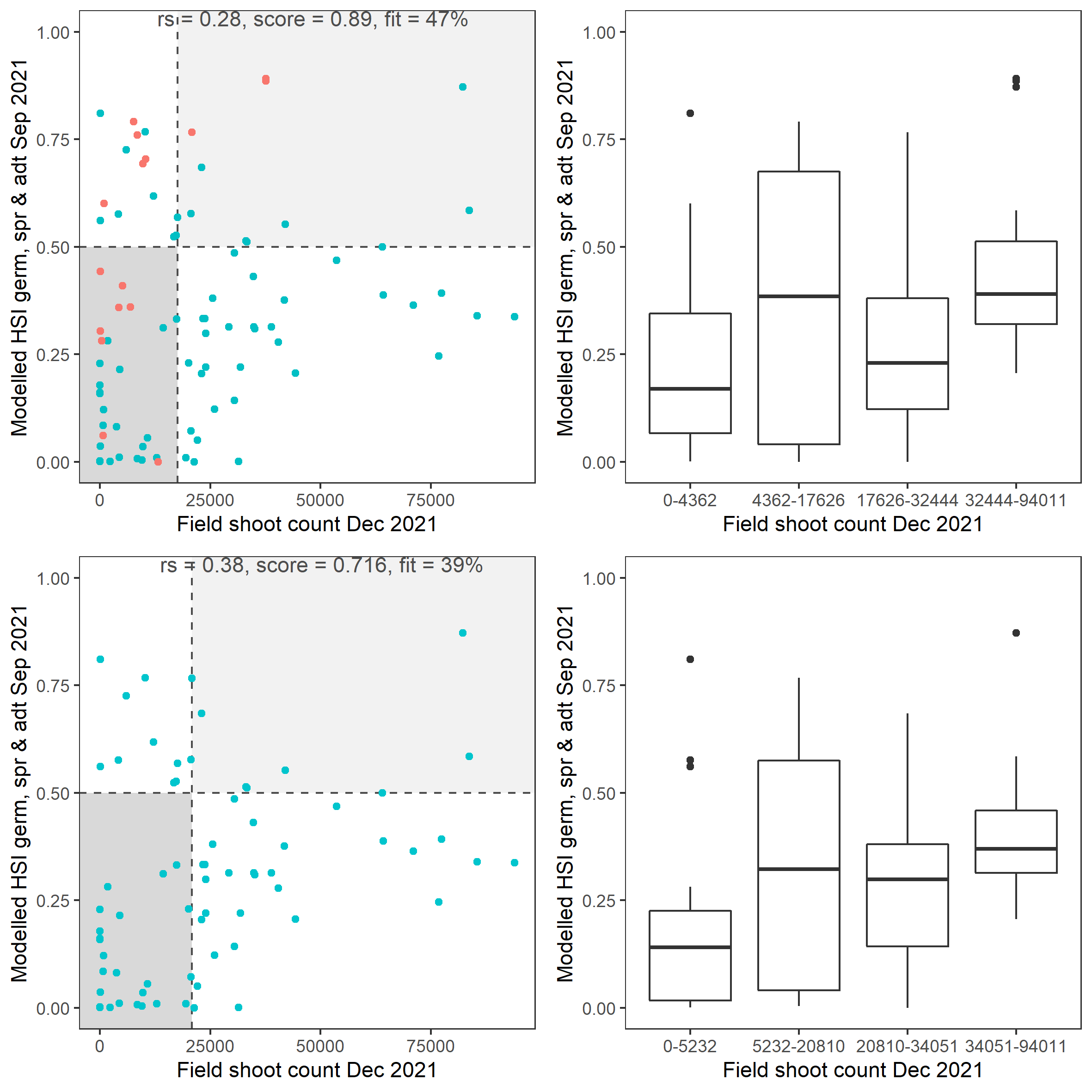
Figure 8.26: Scatter plot and boxplot of average seagrass shoot count per square meter in Dec 2021 versus HSI model output for germination, sprouting and adult growth integrated over Jan - Sep 2020. Top panel: the entire lagoon (red: north, blue: south), bottom panel: south lagoon. An HSI of 0 represents unsuitable habitat conditions, while an HSI of 1 represents optimal conditions. Vertical dashed line: median count; horizontal dashed line: HSI = 0.5, above which the habitat is classified as ‘preferred habitat’; points within light shaded area: True Positive; points within dark shaded area: True Negative.
vi. Field flower count Dec 2021 (obs) vs. HSI sexual Dec 2021 (model)
Average number of Ruppia flowers per square meter recorded in Dec 2021 (reproductive period) were compared with overall HSI for sexual reproduction in 2021 (Figure 8.27 and 8.28). The validation scores of 2021 were lower than that of 2020, possibly due to the environmental conditions experienced in winter-spring 2021 (including unusually cool and wet conditions), which may have caused a delay in the Ruppia life cycle (Waycott 2022, pers. comm.). Overall very few flowers were recorded in the 2021 reproductive period. It was speculated that flowering may be triggered by warming temperature (Waycott 2022, pers. comm.), the threshold of which remains unclear (in the current model the temperature threshold for flowering is assumed to be the same as vegetative growth).

Figure 8.27: Average Ruppia flower count per square meter in Dec 2021 (circles) overlaid on HSI model output for overall sexual reproduction integrated over Jan – Dec 2021. An HSI of 0 (dark purple) represents unsuitable habitat conditions, while an HSI of 1 represents optimal conditions (yellow).
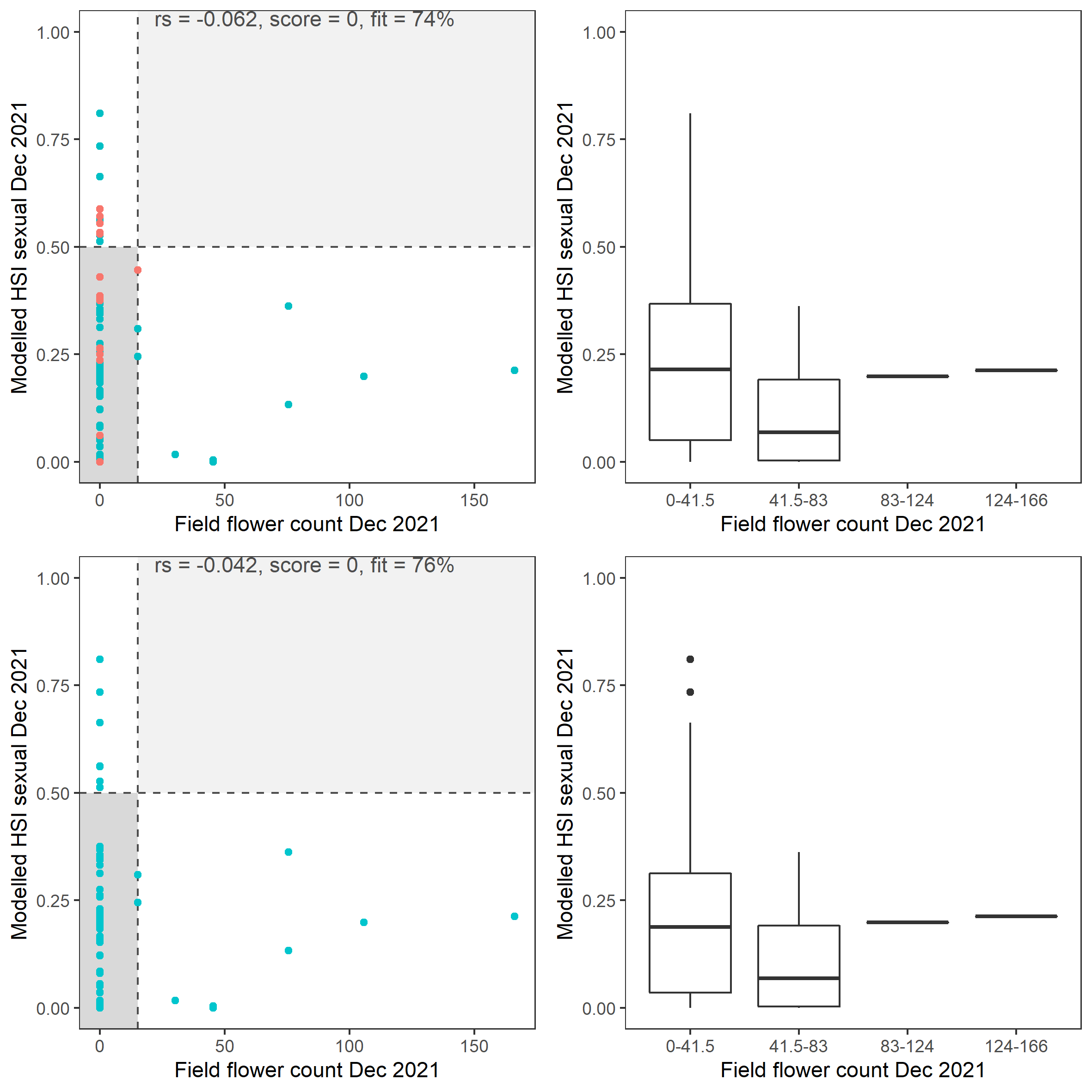
Figure 8.28: Scatter plot and boxplot of average Ruppia flower count per square meter in Dec 2021 versus HSI model output for overall sexual reproduction integrated over Jan – Dec 2021. Top panel: the entire lagoon (red: north, blue: south), bottom panel: south lagoon. An HSI of 0 represents unsuitable habitat conditions, while an HSI of 1 represents optimal conditions. Vertical dashed line: median count; horizontal dashed line: HSI = 0.5, above which the habitat is classified as ‘preferred habitat’; points within light shaded area: True Positive; points within dark shaded area: True Negative.
vii. Field seed count Dec 2021 (obs) vs. HSI sexual Dec 2021 (model)
Average number of Ruppia tuberosa seeds per square meter recorded in Dec 2021 (reproductive period) were compared with overall HSI for sexual reproduction in 2021 (Figure 8.29 and 8.30). It was expected that seed prediction may not be accurate this year since flowering activity was markedly delayed and would not have yet set seed in Dec.
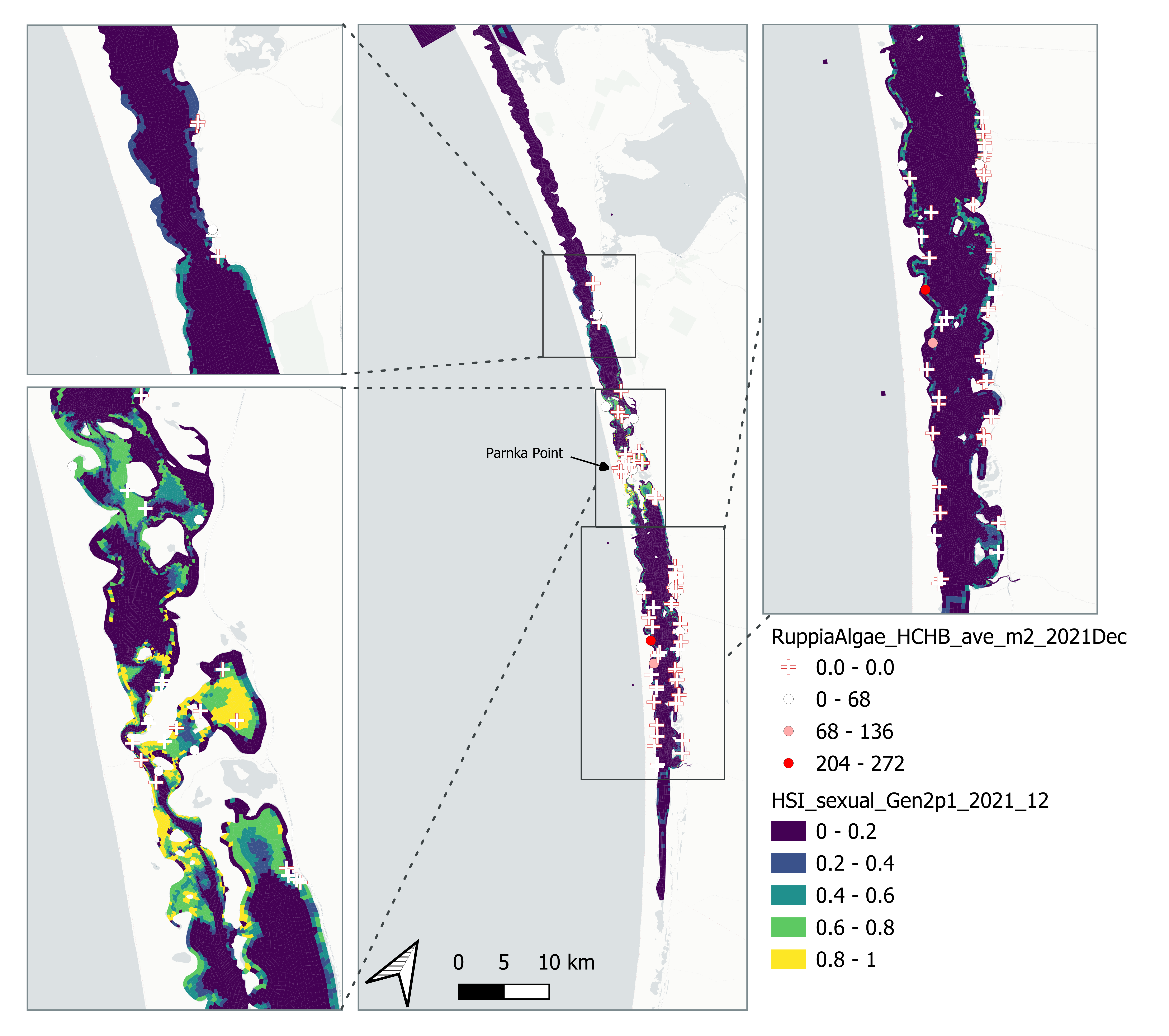
Figure 8.29: Average Ruppia tuberosa seed count per square meter in Dec 2021 (circles) overlaid on HSI model output for overall sexual reproduction integrated over Jan – Dec 2021. An HSI of 0 (dark purple) represents unsuitable habitat conditions, while an HSI of 1 represents optimal conditions (yellow).
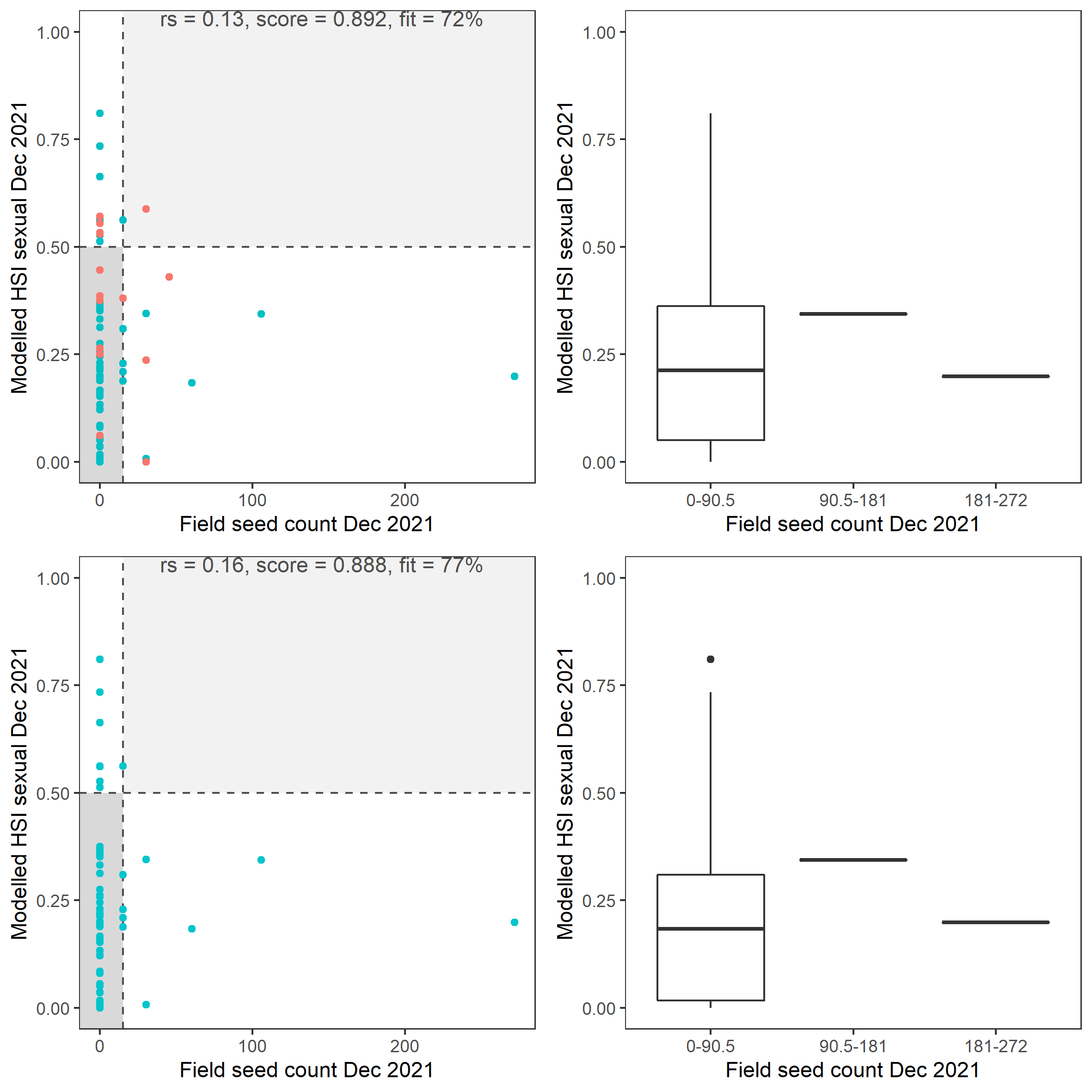
Figure 8.30: Scatter plot and boxplot of average Ruppia tuberosa seed count per square meter in Dec 2021 versus HSI model output for overall sexual reproduction integrated over Jan - Dec 2021. Top panel: the entire lagoon (red: north, blue: south), bottom panel: south lagoon. An HSI of 0 represents unsuitable habitat conditions, while an HSI of 1 represents optimal conditions. Vertical dashed line: median count; horizontal dashed line: HSI = 0.5, above which the habitat is classified as ‘preferred habitat’; points within light shaded area: True Positive; points within dark shaded area: True Negative.
viii. Field turion count Dec 2021 (obs) vs. HSI asexual Dec 2021 (model)
Average number of Ruppia turion (type I and II) per square meter recorded in Dec 2021 (reproductive period) were compared with overall HSI for asexual reproduction in 2021 (Figure 8.31 and 8.32). The overall distribution of turions agreed with model prediction in that more turions were found around the middle lagoon and northern half of south lagoon, where HSI were higher.
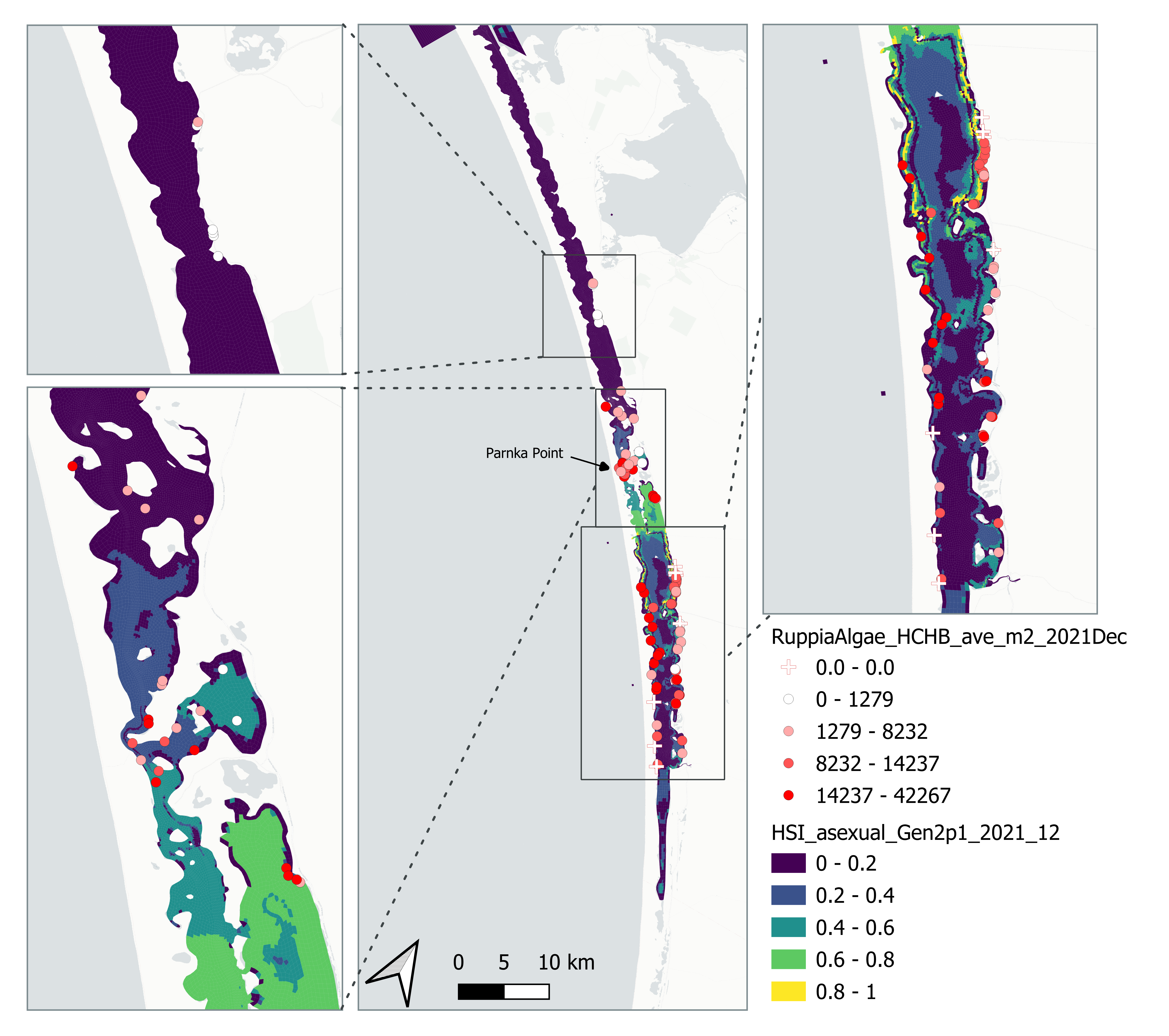
Figure 8.31: Average Ruppia turion count per square meter in Dec 2021 (circles) overlaid on HSI model output for overall asexual reproduction integrated over Jan – Dec 2021. An HSI of 0 (dark purple) represents unsuitable habitat conditions, while an HSI of 1 represents optimal conditions (yellow).
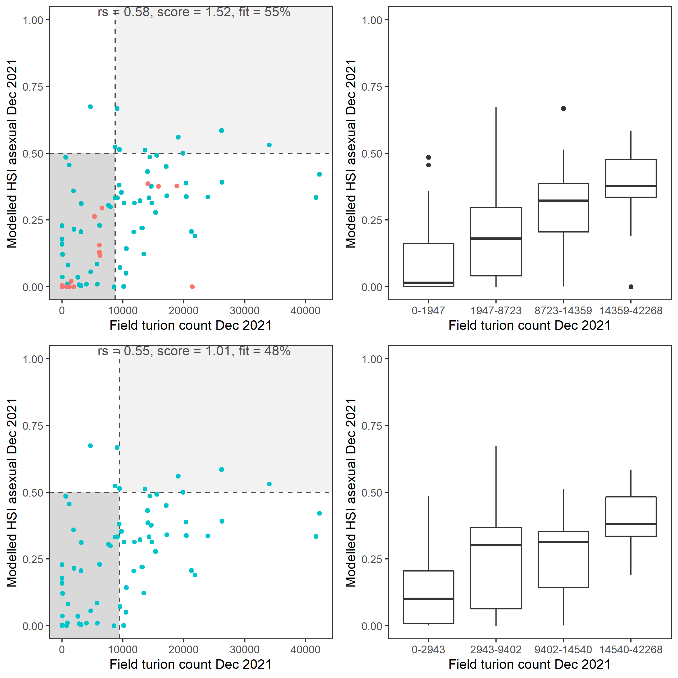
Figure 8.32: Scatter plot and boxplot of average Ruppia turion count per square meter in Dec 2021 versus HSI model output for overall asexual reproduction integrated over Jan - Dec 2021. Top panel: the entire lagoon (red: north, blue: south), bottom panel: south lagoon. An HSI of 0 represents unsuitable habitat conditions, while an HSI of 1 represents optimal conditions. Vertical dashed line: median count; horizontal dashed line: HSI = 0.5, above which the habitat is classified as ‘preferred habitat’; points within light shaded area: True Positive; points within dark shaded area: True Negative.
8.1.6 Summary
We undertook an extensive review of historical and HCHB Ruppia
monitoring data and literature review on environmental influences
including the effect of macroalgae on all Ruppia life-stages. We also
conducted statistical analyses on Ruppia phenology and distribution
data in relation to salinity, water depth and macroalgae abundance.
Based on literature review, data analyses and on-going model assessment,
we have developed the Ruppia Gen 2.0 model by 1) refining relevant
environmental threshold parameters and time windows for all Ruppia
life-stages, with a new life-stage function (turion viability) added to
the model; 2) improving life-stage integration approach in the model. We
have also for the first time developed an approach for validating model
output against field data. Model performance was overall
satisfactory, where areas with higher HSI predicted by the model aligned
with higher abundance recorded in the field in most cases.
More recently, the Gen 2.1 model was tested against the Gen 2.1 hydrodynamic model with the refined mesh.
Overall, Gen 2.1 model produced similar Ruppia HSI predictions to Gen
2.0, with some improvements in error metrics for some life-stages in
2021. The additional two error metrics calculated, fit and score, suggested that the model can predict True Positive and True Negative reasonably well with an average overall goodness-of-fit of 65% for all life-stages across both years, and that model predictions were informative (score > 1) for all life-stages except for shoot and flower in 2021.
The year-to-year variability in model performance, however, indicates that there were likely environmental factors influencing the distribution and abundance of Ruppia and its life phases that were not accounted for in the model, such as environmental cues for flowering event, which may include elevated temperature and photoperiod. Similar for other life stages, statistical analysis conducted on HCHB survey data showed that only a small portion of the variances in the distribution of seagrass biomass (23%), Ruppia seeds (6.8%) and turion (13%) could be explained by salinity, depth, elevation, algae biomass, and distance to Murray Mouth (Lewis et al., 2022). Although the unexplained variances remain a knowledge gap, it is important to note that our Ruppia model focuses on the potential suitability of habitats based on environmental factors and does not take into account biotic interactions such as foraging by birds. Our model focuses on the annual life cycle of Ruppia, while it was observed during the HCHB surveys that there exists a perennial Ruppia community in the Coorong (Lewis et al., 2022) which may cause some mismatch between the modelled and observed Ruppia presence. However what factors contribute to Ruppia community persisting through the aestivation period is unclear and could potentially be integrated into our model in the future.
8.2 Habitat modelling - Fish
8.2.1 Overview
The high salinity values experienced in times of low freshwater flows challenges the fish populations that inhabit the lagoon. As an indicator of suitable conditions, the fish model calculates probabilities of habitat suitability for juveniles of seven key species, mulloway (Argyrosomus japonicus), black bream (Acanthopagrus butcheri), greenback flounder (Rhombosolea tapirina), yelloweye mullet (Aldrichetta forsteri), congolli (Pseudaphritis urvillii), Tamar goby (Afurcagobius tamarensis) and smallmouth hardyhead (Atherinosoma microstoma), based on laboratory experiment-derived salinity thresholds (Table 8.11. from @mcneil2013).
8.2.2 Model description: Fish HSI
The model adopts a seasonal effect by account for temperature sensitivity to the salinity thresholds (higher salinity tolerance at lower temperatures), according to functions and parameters described below. It is computed as:
\[\begin{equation} Fish\: HSI =\left\{ \begin{array}{@{}ll@{}} 1, & 0 \le S \lt S_{c10} \\ \frac{S_{c50}-S}{S_{c50}-S_{c10}}, & S_{c10} \le S \lt S_{c50}\\ 0 & S\ge S_{c50}\\ \end{array}\right. \end{equation}\]where \(S\) is salinity \(S_{c50}\) is the temperature-corrected concentration of salinity that kills 50% of the test animals and \(S_{c10}\) is the temperature-corrected concentration of salinity that kills 10% of the test animals. These are based on lethal concentration tests at specific temperatures, and calculated according to:
\[\begin{equation} S_{c10} =\left\{ \begin{array}{@{}ll@{}} LC_{10}^{14}, & 0 \le \bar{T} \lt 14 \\ \frac{LC_{10}^{23}-LC_{10}^{14}}{23-14}(T-14) +LC_{10}^{14} , & 14 \le \bar{T} \lt 23 \\ LC_{10}^{23}, & \bar{T} \ge 23 \\ \end{array}\right. \end{equation}\] \[\begin{equation} S_{c50} =\left\{ \begin{array}{@{}ll@{}} LC_{50}^{14}, & 0 \le \bar{T} \lt 14 \\ \frac{LC_{50}^{23}-LC_{50}^{14}}{23-14}(T-14) +LC_{50}^{14} , & 14 \le \bar{T} \lt 23 \\ LC_{50}^{23}, & \bar{T} \ge 23 \\ \end{array}\right. \end{equation}\]
where \(\bar{T}\) is the monthly average water temperature and the \(LC\) are the experimentally determined salinity concentrations that removed 10 and 50% of the population for the denoted temperatured.
Figure 8.33 shows an example three-dimensional plot of the HSI functions for mulloway. In addition, habitat is deemed unsuitable if water is less than 0.1m deep. The computed habitat suitability index (HSI) ranges between 0 and 1, where 0 represents least suitable and 1 represents most suitable. Details of model description and application are described in Brookes et al. (2022).
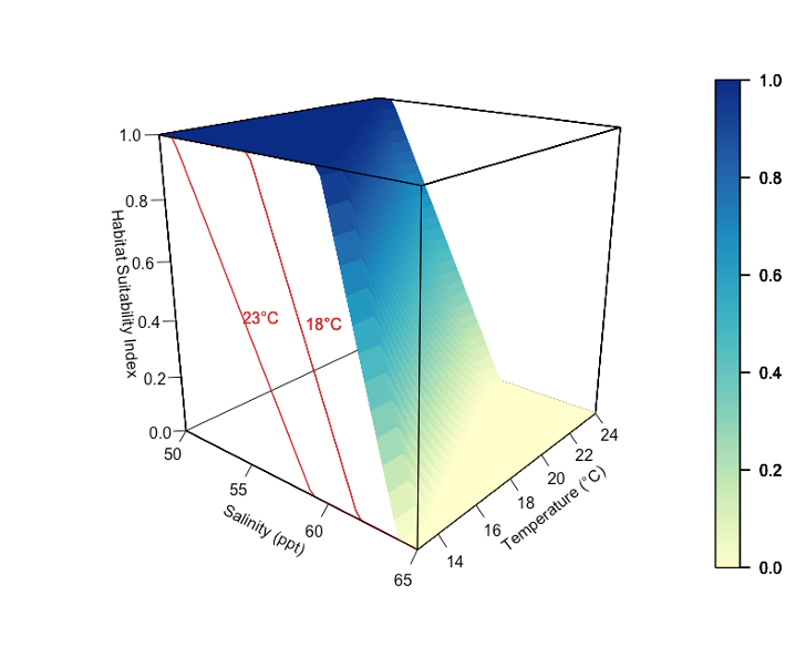
Figure 8.33: Fish Habitat Suitability Index (HSI) surface plot (3D) as a function of salinity tolerance for mulloway, where a HSI value of 1 represents the most suitable conditions and 0 the least suitable. The salinity thresholds are specified as a function of water temperature where fish is able to tolerate higher salinities at lower temperatures. The red lines (2D) show the effect of salinity on HSI at two fixed temperatures
8.2.3 Data availability
Environmental threshold parameter review
The following parameters have been assigned as the temperature and salinity thresholds (Table 8.11).
| Common name | \(LC^{14}_{50}\) | \(LC^{23}_{50}\) | \(LC^{14}_{10}\) | \(LC^{23}_{10}\) |
|---|---|---|---|---|
| Mulloway | 64 | 59 | 60 | 51 |
| Tamar goby | 73 | 71 | 68 | 66 |
| Black bream | 85 | 88 | 79 | 82 |
| Greenback flounder | 88 | 79 | 81 | 73 |
| Yelloweye mullet | 91 | 82.4* | 84 | 68 |
| Congolli | 100 | 94 | 90 | 87 |
| Smallmouth hardyhead | 108 | 108 | 100 | 97 |
8.2.4 Model application and results
The Generation 0 model was run between 2017 - 2020 using the base case and two management scenarios. For details of model application and results please refer to Brookes et al. (2022).