Assessment 3B - Modelling catchment response to climate change
Learning Objectives
The aim of this assessment is to develop your thinking about how we can conceptualise environmental systems in times of change, how different “components” of the environment link together, and to understand approaches to predict changes to the environment brought about by climate change. We look at simple example of a catchment-lake system, but the methods and logic introduced are relevant for how assessments are undertaken to assess how climate change impacts real-world systems.
You will work through the assessment in three parts focused on:
A. Catchment streamflow prediction

B. Lake dynamics

C. Assessing climate change impacts
At the completion of this assessment learners will have demonstrated an ability to;
describe hydrological system dynamics as a mathematical model
quantify and predict hydrological processes under a changing climate
A. Catchment Model
Consider a river basin with 3 sub-catchments, each with a different dominant land use and slightly different climate.
The daily runoff from each sub-catchment, \(Q_i\) (m3/day), can be simply approximated based on the daily rainfall (\(R\)), where \(c\) is the daily runoff efficiency and \(R^{crit}\) is the initial loss threshold (\(m\), this is the amount of rainfall that does not make it to the stream):
The “\(t\)” super- script refers to a “time-step,” usually referring to a single day. The “\(i\)” subscript in the above refers to the catchment index; in other words, \(i=1\) refers to sub-catchment 1.
The total flow (\(Q_{tot}\), m3/day) is calculated by summing the individual sub catchments, however there is an assumed lag time of 1 day for sub-catchment 2 and 2 days lag time for sub-catchment 3:
The time-lag of one day (\(t-1\)) and two days (\(t-2\)), is a way to simply account for the time it takes for water in sub-catchment 2 and 3 to reach to overall catchment outlet, a process we call streamflow routing.
Module Resources
Download the Excel spreadsheet for this assessment by clicking the download button in the tool bar .
Building the model
- Draw by hand the conceptual model of this system.
- Confirm what the indices are referring to in the above equations (\(t\), \(i\)).
- Build the above model in Excel, to predict the individual sub-catchment flows and river basin total flow. Assume basic information as outlined in Table 7 below and the supplied rainfall data for the 3 sub-catchments. Input a guessed value for \(c\) within the range indicated for now.
| Parameters for catchment model: | Sub Catchment 1 (\(i\)=1) | Sub Catchment 2 (\(i\)=2) | Sub catchment 3 (\(i\)=3) |
|---|---|---|---|
| Sub catchment area, \(A\) (km2) | 50 | 100 | 120 |
| Runoff coefficient, \(c\) (range) | 0.2 to 0.5 | 0.1 to 0.4 | 0.1 to 0.3 |
| Initial loss threshold value, \(R_{crit}\) (m) | 0.01 | 0.025 | 0.04 |
| Landuse fraction, \(F\): irrigated dairy | 0.1 | 0 | 0.5 |
| Landuse fraction, \(F\): wheat | 0 | 0.8 | 0.1 |
| Landuse fraction, \(F\): urban | 0.3 | 0 | 0.1 |
| Landuse fraction, \(F\): forest | 0.6 | 0.2 | 0.3 |
Calibrating the model
Now we have the model running, let’s make sure the predicted flows are realistic. Previously we assumed a value of \(c\) for each sub-catchment, but what is the best value for each sub-catchment that would give the most accurate prediction?
- Manually adjust the runoff coefficient values (\(c\)) for each sub-catchment (see possible ranges in table above) until the model best matches the observed data. This process is called “calibration.”
- Plotting the time-series of daily flows is”crowded” and it’s hard to see differences. In this case we therefore do what is called a “cumulative mass-curve.” For this we cumulate the daily flow and plot over time – so it keeps increasing. This is the cumulative mass of water (usually presented in m3) delivered by the catchment. Create a “stacked area plot” of the cumulative flow from each sub-catchment.
Land-use change scenario
Lets assess a land-use change scenario, and see how urbanisation may affect runoff amounts.
- If the total urban area in each sub-catchment expands to 50% (\(F_{urban}=0.5\)), how would this affect the overall amount of water discharged?
To compare scenarios we could plot time-series of streamflows with multiple series on a single plot. As above, we can more easily compare scenarios using the cumulative mass plot, as they will start to diverge and the differences will stand out more clearly.
- Prepare a cumulative time-series of water from the orginal calibrated model, and the urban land-use change scenario. Quantify the difference between the two in terms of annual water volume for each catchment.
B. Lake system model
The catchment we have simulated above discharges its water into a lake system located at the low point of the landscape. This includes two main lakes which are situated in sequence. Aside from the catchment river inflow, the lakes receive and lose water from various hydrological pathways The lakes can fill up and overflow, above a certain critical lake height, and overflow water from the initial lake flows to the downstream lake.
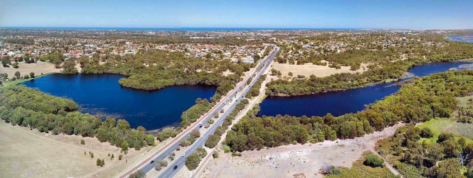
Figure 30: Two-lake system
Given the position of upper lake in the landscape it is likely to be a through-flow lake, so we also include terms for groundwater outflow, connecting the two lakes. We’ll assume that groundwater inflow is determined by the regional groundwater gradient which is relatvely stable so that we can use a constant value. For groundwater outflow, we can use the same approach as we used in Exercise 5 (Simple lake model), where infiltration was a function of water level in the lake.
Bearing this in mind, the water balance equation describing the change in lake storage (\(S\), \(m^3\)) of the upper lake is:
\[\begin{equation} \frac{dS_{upper}}{dt}= Q_{tot} +\underbrace{ (R - E -kh_{upper} ) A_{upper} }_{\text{upper lake fluxes}} - Q_{out_{upper}} \tag{14} \end{equation}\] \[\begin{equation} \frac{dS_{lower}}{dt}= Q_{out_{upper}} + \underbrace{ kh_{upper} A_{upper} }_{\text{gw from upper -> lower}} + \underbrace{ (R - E - kh_{lower}) A_{lower} }_{\text{lower lake fluxes}} - Q_{out_{lower}} \tag{15} \end{equation}\]
wher \(R\) is the precipitation (\(m/day\)) falling on the relevant lake (precipitation rate x lake area, \(A\)), \(Q_{tot}\) is the inflow (discharge) rate from the catchment (\(m^3/day\)), \(Q_{out_{upper}}\) is the overflow from the upper to the lower lake, \(E\) is the evaporation rate (\(m/day\)) and the \(khA\) terms reflect the groundwater seepage associated with each of the lakes.
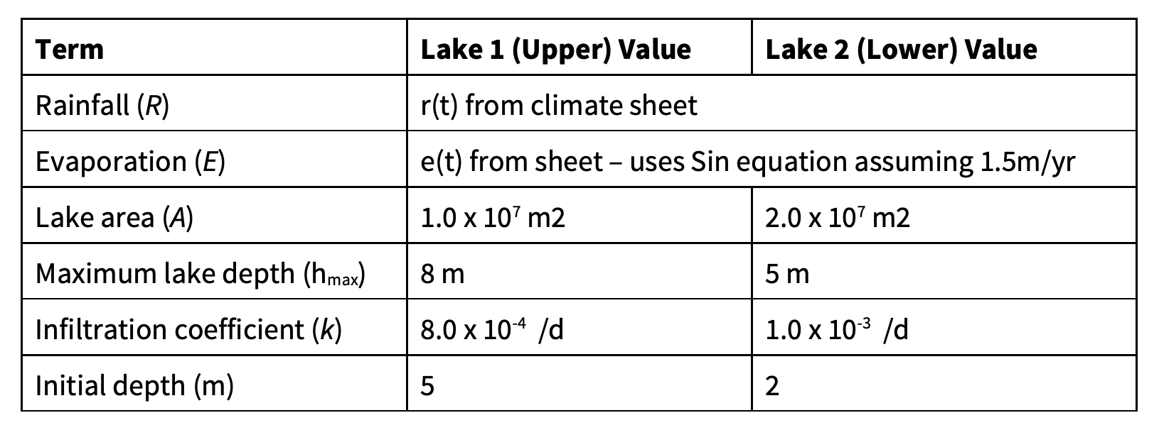
Figure 31: Model parameters for lake system water level simulation
With these we can model the water storage in the two lakes. Start with the template spreadsheet provided. You can use the daily rain and evaporation (data provided) to drive this model, but you will need to ensure you have consistent units across terms (i.e. all rates are /d, not a mix of /d and /y, and note that volumes are different from lengths!).
We will assume that the sides of the lakes are steep so that lake surface area is independent of water level height. Therefore, water level is related to the storage volume in the lake according to:
To start the simulation we must use an initial lake water level, as provided in the details below (Table 4), to get the starting lake storage, \(S^{t=0}\) or \(S^{0}\).
The outflow (overflow) of each lake only occurs when the lake water level exceeds the maximum depth, which are denoted \(h^{max}_{upper}\) and \(h^{max}_{lower}\). In general, for either lake:
where \(h^{t*}\) is the estimate of what the daily water level would be prior to computing \(Q_{out}\) (i.e., an interim value). Note that when applying this, and \(IF\) statement can be used to compute the equation above.
The rate of potential evaporation, \(E_{p_{annual}}\) \((m/yr)\), at the chosen location varies seasonally - more in summer and less in winter. It is rare to measure evaporation so instead we can rely on the annual rate of potential evaporation, and spread it over a year using a sine wave. The sine wave, is tailored to ensure the peak is in summer and the trough is in winter, and that the sum of the daily evaporation rates adds to the annual total:
This is depicted visually in Figure 32, which is incorporated in the provided data sheet with typical parameters for Perth conditions.
Figure 32: Potential evaporation rate sine wave function used to capture seasonal variation in lake evaporation.
Building the model
Now we have established the background, start building the model by following these steps:
- Sketch the described system, setting the context and using the notation above.
- Write out the above two equations using “difference” notation (i.e., \(S^{t+1}_{lower} = S^t_{lower} + R^t...\) ).
- Open the LakeModel spreadsheet and finish the columns for the Upper Lake, using the below settings in Table 2 (change the red numbers to match Table 4).
- Plot the Upper Lake storage and water depth over time. Now also plot the water fluxes.
- Once this lake looks good, implement the columns needed for resolving the Lower Lake, based on Eq 19 above.
Assessing the model
- Change the settings (model parameters) to see the sensitivity to leakage (\(k\)) and maximum lake depth (\(h_{max}\)).
- Would increasing or decreasing the surface area of Lower Lake help stabilise the water level?
- Use the model to demonstrate an alternate scenario of lake management – how would this change the lake water levels?
- How realistic is this model and what changes could you make if you were asked to improve it?
C. Climate change impact assessment
In the final part of this assessment, we continue modelling calculations that we have developed previously with one addition: we use your models to predict the effects of a changing climate. Lake water quality has been highlighted as being sensitive to climate change (Trolle et al., 2011). Within Western Australia, a significant decline in rainfall has been observed (e.g., https://water.wa.gov.au/planning-for-the-future/allocation-plans/managing-water-in-a-changing-climate/climate-change-impacts-on-the-south-west)
Read the document ‘Climate analyses for south-west Western Australia’ (CSIRO, 2010) to learn about the projected climate changes for the coming decades, the various scenarios proposed and the different models that are synthesised in the report. For example, look at Sections 4.5.1 Rainfall Change and 4.5.2 Areal Potential Evaporation show predicted rainfall and evaporation changes for the year ~2030.
Use your judgement to select seasonal and annual trend changes, for example, one model may predict a 2% decrease in spring rainfall and a 3% increase in evaporation for the area around Perth. Alter your climate forcing data so that it reflects one of the climate models forecast. Recalculate the water balance for 2030 to 2033 with your new rainfall and evaporation forcing. This is essentially a new scenario of your model.
When describing the methods for this climate change assessment, explain the methods you used to obtain the climate change trend from the CSIRO report, and then the approach to alter the climate forcing in the model.
When describing the results of the climate change impacts, explain what the differences were between the base case and the projected scenarios. Create a set of figures that show the differences between the base case scenario and any future scenarios for key catchment and lake results.
When interpreting the results, consider:
• how your results match the rest of the climate literature that you have researched,
• positive or negative changes for future lake ecosystems in 2033,
• the benefits of regional and global climate models,
• the relative merits of simple bucket models and complex general circulation models,
• any other effects of increased temperature that are not captured in this model,
• how the model could be improved, and the next steps that future modellers could carry out.
Submission
Your submission is a single report based building on all three parts (A, B and C) listed above. Use the questions in each part as a guide to the ideas that should be included in your report. You can expect to end up with about 10 pages for this report.
Your report should address:
• the scientific aspects associated with catchment and lake assessment, and
• the technical and practical aspects of numerical modelling.
The structure of the report should be as follows:
Introduction : Include just the background information that is necessary to understand your aim. This should relate to assessment of land-use change and climate change. Introduce all three parts of the assessment together in a nicely connected way within the one introduction. Include an aim, and a hypothesis if you can. Include conceptual diagrams if they help explain the background.
Methods : Explain what you did so that someone else could repeat it Separate the three parts within this one Methods section, using sub-sections for the catchment, lake and climate aspects. Use past tense and a passive voice. Show the model equations and define all parameters used. Including any sources for parameter values or estimates found in the literature. You can include conceptual diagrams to help explain the methods
Results : Report the numbers, trends or other findings you calculated. Include figures if they help you explain the results, for example, time series. Large tables of results are often better placed in an Appendix. Separate the three parts within this one Results section. Remember to label all of your axes with the correct units, provide a legend only if necessary, and add a caption underneath the figure. Don’t add a title on a figure (use a caption).
Discussion : Assess the ability of the model to capture this system. You may wish to consider - - The suitability of the conceptual model (is it flawed or robust?) - The model equations - The software used - The uncertainty of the parameters - How managers could use this to help adapt to a changing climate
Conclusion :Give a general conclusion of all three parts of the assessment. Connect your results to your aims. Connect your results to the rest of your background reading.
References : Follow the unit style and use a consistent format throughout.