Exercise 2 - Streamflow analysis
In this exercise we understand how to generate streamflow data, and then how to use it characterise variability in stream discharge rates.
Learning Objectives
By the end of this exercise learners will be able to:
- Describe and utilize standard approaches for measuring or estimating streamflow
- Characterize stream hydrology through the analysis of streamflow data
Measuring Stream Velocity & Discharge
The process of measuring stream flow (volume rate of flow), or discharge, is called stream gauging. There are numerous methods of stream gauging, including direct methods, such as volumetric gauging, and dilution methods, as well as indirect methods involving stage-discharge relations, or rating curves. Since the velocity of a stream varies with depth and width across a stream, it is important to understand what it is you want to measure when choosing a stream gauging method. If you are interested in stream surface velocity, a simple float method would work well. This method involves throwing some buoyant, highly visible object into the stream and measuring the time it takes to float a known distance. If you are interested in obtaining a more accurate stream discharge measurement, the velocity-area method is your method of choice.
Stream flow (discharge) can be measured based on two fundamental methods, which are each expanded upon below (refer to lecture 3 for details). The first requires a direct measurement of velocity, whereas the second is an approximation based on stream-bed slope and geometry.
Flow Rate: Velocity-Area Method
Flow estimates in natural streams and artificial channels under steady (no change in depth with time) and uniform (no change in depth with space) conditions can be computed by the product of mean flow velocity (integrated in depth and across the channel) and the cross-sectional area of flow. The equation \(Q = V * A\), were \(V\) (m/s) is the mean velocity and \(A\) (m2) is the flow (or water) cross-sectional area is used for this purpose. Large streams and rivers, a section control is needed to generate the “rating curve” thus establishing a relationship between water stage height (\(H\)) and flow discharge (\(Q\)). In this case, both flow velocity measurements and cross-sectional areas are needed.
Discharge using the Velocity-Area method is measured by integrating the area and velocity of each point across the stream. The channel or stream is divided into sections based on where the velocity and stage height measurements were taken in the cross-section of the stream/channel. The flow velocity is measured using a current meter (i.e. propeller, electromagnetic, ultrasonic, and Doppler).
The discharge is computed using:
where \(n\) is the number of vertical for measuring velocities, \(V_{i}\) is the mean velocity value for vertical \(i\) (m/s) and \(\text{Area}_i\) is the cross-sectional area around vertical \(i\) (m2). The cross-sectional area is best estimated by treating the sections as rectangles, trapezia or triangles.
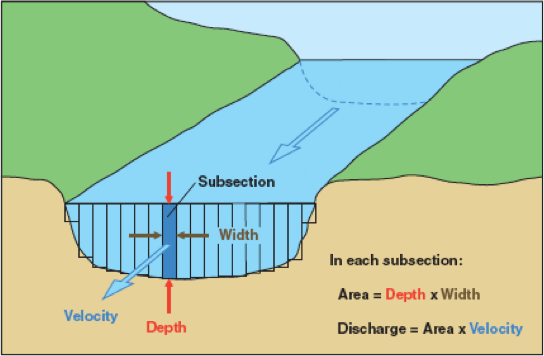
Figure 2: Current-meter discharge measurements are made by determining the discharge in each subsection of a channel cross section and summing the subsection discharges to obtain a total discharge.
To measure stream velocity we can utilise a “swoffer” – a pole with a propeller on the end with an electronic logger recording the rotations. A current meter is so designed that its rotation speed varies linearly with the stream velocity at the location of the instrument.
A more modern alternative is an “ADV” (Acoustic Doppler Velocimeter). This relies on a method where it looks at the scatter of sound waves rebounding of particles/bubbles in the water, and based on the “Doppler effect” (recall the sound of a train changing pitch as it moves past you), it can compute the water velocity.
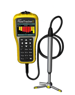
Figure 3: An ADV - used to measure stream velocity.
Activity: Watch the videos below showing the principles of how to measure the velocity of water. Then calculate the streamflow at the two sites in Table. The “section” column tells you nominally where you are across the x-section, the “width” column is the actual width of flow you should use in your calculations. Each velocity and depth measurement was made at the distance across the stream reported in the “distance” column.
Does the wider stream section have more streamflow? Is this what you would have expected?
Site 1 is upstream of Site 2, did the flow increase or decrease downstream? What might have caused this change in flow?
| Site | Total Width (m) | Section (m) | Distance (m) | Depth (m) | Width (m) | Velocity (m/s) |
| Site 01 | 3.8 | 0-0.5 | 0.5 | 0.29 | 0.75 | 0.044 |
| 0.5-1 | 1 | 0.34 | 0.5 | 0.215 | ||
| 1-1.5 | 1.5 | 0.26 | 0.5 | 0.227 | ||
| 1.5-2 | 2 | 0.3 | 0.5 | 0.247 | ||
| 2-2.5 | 2.5 | 0.25 | 0.5 | 0.232 | ||
| 2.5-3 | 3 | 0.2 | 0.5 | 0.091 | ||
| 3-3.8 | 3.5 | 0.11 | 0.55 | 0.06 | ||
| Site 02 | 3 | 0-0.5 | 0.5 | 0.33 | 0.75 | 0.445 |
| 0.5-1 | 1 | 0.33 | 0.5 | 0.399 | ||
| 1-1.5 | 1.5 | 0.35 | 0.5 | 0.277 | ||
| 1.5-2 | 2 | 0.29 | 0.5 | 0.388 | ||
| 2-3 | 2.5 | 0.23 | 0.75 | 0.424 |
Flow Rate: Manning’s Formula
Manning’s formula for estimating streamflow (in m3s-1) from basic channel geometry, slope and roughness is:
Where: \(A\) is the channel cross-sectional area (m2) ; \(R\) is the hydraulic radius given by \(\frac{A}{P}\) ; \(P\) is the wetted perimeter (i.e. bed plus banks; m); \(S\) is the channel slope (m/m); \(n\) is Manning’s ‘n’ (which is an empirical roughness coefficient).
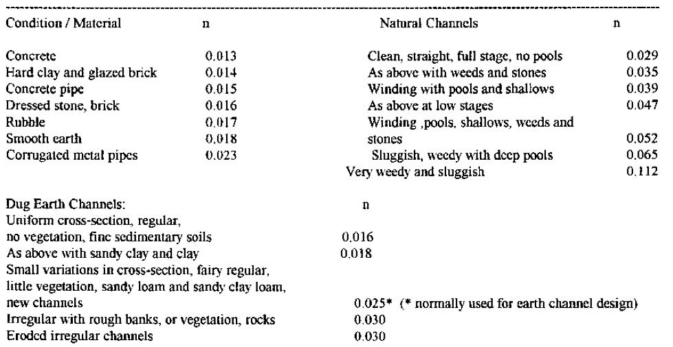
In practice, when you are in the field the bottom slope (\(S\)) will be measured by using a differential GPS (DGPS). You also need to measure the ‘wetted perimeter’ (\(P\)) of the channel and the cross sectional area (\(A\)). The roughness coefficient (\(n\)) should be assumed from the literature, based on your observations or the stream and a table like the one below, or here, or here, or here.
Activity: For this activity we will use some of the same measured data that we used for the velocity-area method. Those measurements were taken on Carey Brook, a tributary to the Donnelly River in south-west Western Australia (near Pemberton). You have already calculated the total area (sum the individual areas calculated in the velocity-area method). Draw a scale diagram of your chosen cross-section to estimate the wetted perimeter. Use the slope over the 5.2 km of Carey Bk between the main highway (25 m AHD) and where it flows into the Donnelly River (7 m AHD). Now you just need a roughness parameter, Manning’s \(n\), and you can solve Equation (3).
How does this streamflow estimate compare to the answer you got using the velocity-area method above?
How sensitive is your answer to the value of Manning’s \(n\)?
Making Sense of Streamflow Data
The first step in any hydrologic data analysis project is to gather the data and relevant background information on your catchment of interest. In Western Australia the WIR website contains all of the data and information you need, and we will use this in our future assignments. All states/countries have something similar; the USA has one of the best examples through the USGS NWIS website.
)](images/surface_hydrology/picture5.jpeg)
Figure 4: The Avon River, Western Australia
Hydrologic analyses are almost always conducted for “water years” not calendar years. In the Northern Hemisphere. A water year begins on October 1 and ends September 30 . In the Southern Hemisphere it Starts May 1 and ends April 30, though this can be region specific.
Activity: Go to the WIR web link, and download the continuous flow data for the Swan River “Walyunga” gauge (616011). In Excel, explore the data. Create a hydrograph comparing discharge between a wet year and a dry year (i.e. plot two years on a common x-axis. Use “hydrologic years” rather than calendar years. Label accordingly.
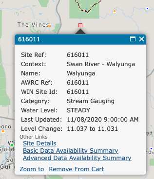
Figure 5: Navigate to the ‘Walyunga’ guage (616011)
Flow Duration Curves
What is it?
The flow duration curve is a plot that shows the percentage of time that flow in a stream is likely to equal or exceed some specified value of interest. For example, it can be used to show the percentage of time river flow can be expected to exceed a design flow of some specified value (e.g., 20 m3/s), or to show the discharge of the stream that occurs or is exceeded some percent of the time (e.g., 80% of the time).
How is it calculated?
The basic time unit used in preparing a flow-duration curve will greatly affect its appearance. For most studies daily discharges are used. These will give a steep curve. When the mean flow over a long period is used (such as mean monthly flow), the resulting curve will be flatter due to averaging of short-term peaks with intervening smaller flows during a month. Extreme values are averaged out more and more, as the time period gets larger (e.g., for a flow duration curve based on annual flows at a long-record station).
Step 1: Sort (rank) daily discharges for period of record from the largest value to the smallest value, involving a total of \(n\) values.
Step 2: Assign each discharge value a rank (\(M\)), starting with 1 for the largest daily discharge value.
Step 3: Calculate exceedence probability (\(P\)) as follows:
Where, \(P\) = the probability that a given flow will be equaled or exceeded (% of time), \(M\) = the ranked position on the listing (dimensionless), and \(n\) = the number of events for period of record (dimensionless).
Activity: Follow the above steps using the 616011 gauge data to create your own flow duration curve.
What does this particular information tell you about your stream?
A flow duration curve characterizes the ability of the basin to provide flows of various magnitudes. Information concerning the relative amount of time that flows past a site are likely to equal or exceed a specified value of interest is extremely useful for the design of structures on a stream. For example, a structure can be designed to perform well within some range of flows, such as flows that occur between 20 and 80% of the time (or some other selected interval).
The shape of a flow-duration curve in its upper and lower regions is particularly significant in evaluating the stream and basin characteristics. The shape of the curve in the high-flow region indicates the type of flood regime the basin is likely to have, whereas, the shape of the low-flow region characterizes the ability of the basin to sustain low flows during dry seasons. A very steep curve (high flows for short periods) would be expected for rain-caused floods on small watersheds. Snow-melt floods, which last for several days, or regulation of floods with reservoir storage, will generally result in a much flatter curve near the upper limit. In the low-flow region, an intermittent stream would exhibit periods of no flow, whereas, a very flat curve indicates that moderate flows are sustained throughout the year due to natural or artificial streamflow regulation, or due to a large groundwater capacity which sustains the base flow to the stream.
An example, properly formatted flow duration curve is shown below (Figure 6).
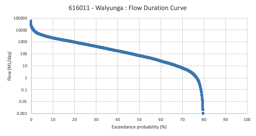
Figure 6: Aproperly formatted flow duration curve
Flood Frequency Analysis
What is it?
Flood frequency analyses are used to predict design floods for sites along a river. The technique involves using observed annual peak flow discharge data to calculate statistical information such as mean values, standard deviations, skewness, and recurrence intervals. These statistical data are then used to construct frequency distributions, which are graphs and tables that tell the likelihood of various discharges as a function of recurrence interval or exceedence probability.
Flood frequency distributions can take on many forms according to the equations used to carry out the statistical analyses. Four of the common forms are: Normal Distribution; Log-Normal Distribution; Gumbel Distribution; and Log-Pearson Type III Distribution. Each distribution can be used to predict design floods; however, there are advantages and disadvantages of each technique.
While the log Pearson Type III distribution is the recommended technique, its application is a bit more complex than we are going to undertake for this class. Instead, we will use the older Weibull plotting position method.
Flood frequency information can be determined from knowledge of the peak discharge (highest discharge) in any given year provided enough years of information has been collected. This allows one to relate the expected recurrence interval for a given discharge, and determine the probability that a flood of a given discharge will occur in any given year. The recurrence interval for a given discharge can be calculated by first ranking the discharges.
Activity: In the Table below for “Big River,” fill in the Rank
column. To do this, enter a 1 for the maximum discharge that has
occurred during the 20 years of available data. The second highest
discharge will be given a rank of 2, etc. with the lowest discharge
given a value of 20.
| Date | Maximum Discharge (m3/s), \(Q\) | Rank, \(m\) | Recurrence Interval, \(R\) |
|---|---|---|---|
| 28-Feb-86 | 1410 | ||
| 4-Mar-87 | 2890 | ||
| 22-Mar-88 | 1850 | ||
| 3-Mar-89 | 800 | ||
| 1-Feb-90 | 1000 | ||
| 12-Apr-91 | 692 | ||
| 4-Apr-92 | 1350 | ||
| 2-May-93 | 1200 | ||
| 16-Mar-94 | 850 | ||
| 6-Jul-95 | 2400 | ||
| 21-Feb-96 | 890 | ||
| 30-Jan-97 | 1480 | ||
| 16-Mar-98 | 1500 | ||
| 21-Feb-99 | 1300 | ||
| 12-May-00 | 1700 | ||
| 8-Apr-01 | 2200 | ||
| 1-Mar-02 | 1830 | ||
| 8-Feb-03 | 1120 | ||
| 12-Mar-04 | 750 | ||
| 6-Mar-05 | 1250 |
After you have filled in the Rank column, you can now calculate the
recurrence interval for each peak discharge. The recurrence interval,
\(R\), is given by the Weibull Equation:
where \(n\) is the number of years over which the data was collected (20 years in this case), and \(m\) is the rank of each peak discharge. Use this equation to calculate the recurrence interval for each peak discharge.
Next, use the graph below (or Excel) to plot a graph of discharge (on the y-axis) versus recurrence interval (on the x-axis). Note that the x-axis must be a logarithmic scale. If drawig by hand you should try to estimate as best you can where the data point will fall between the lines on the graph. Once you have plotted the points use a ruler to draw the best fit straight line through the data points (lay a ruler on the graph and try to draw a line that most closely approximates all of the data points). Do not draw lines that connect individual data points. If you are plotting in Excel you will fit a linear trendline.
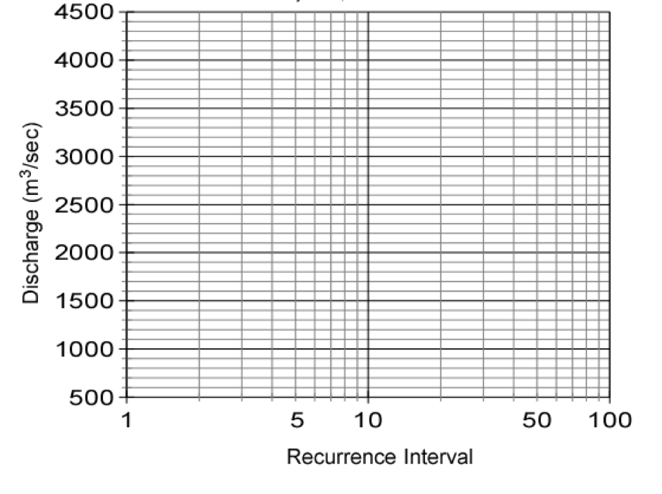
By extrapolating your line on the graph, determine the peak discharge expected in a flood with a recurrence interval of 50 years and 100 years. These are the discharges expected in a 50 year flood and a 100 year flood.
The annual exceedence probability, \(P_{e}\), is the probability that a given discharge will occur in a given year. It is calculated as the inverse of the recurrence interval, \(R\):
Thus, the probability that a flood with a 10 year recurrence interval will occur in any year is 1/10 = 0.1 or 10%. What are the probabilities that a 50 year flood and a 100 year flood will occur in any given year?
Optional Extra: Repeat the above flood frequency analysis using the 616011 Walyunga data set that you downloaded in Excel (Hint, use a pivot table and the max option to get the annual maximum discharge).