Exercise 5 - Simple lake model
Introduction
In this exercise you will use a simple “bucket” storage model of how a lake level fluctuates through time. You can use simple iterative schemes for solving differential equations as a means of modelling environmental systems. The most straightforward numerical approaches involve repetition or iteration of a calculation to evaluate how the system changes through time or space. Here we are completing a modified version of an exercise from Wainwright and Mulligan (2002) (see p38). Similar types of models have been used for paleo-environmental reconstructions (Bradley 1999) and in hillslope hydrology (Dunin 1976), where the bucket represents the ability of soil to hold water. This type of approach can also be used to simulate solute concentrations, which is particularly useful for quantifying exchanges between surface water and groundwater (Cook 2013).
Learning Objectives
By the end of this exercise learners will be able to:
- Understand the role of differential equations in decribing hydrologic systems
- Predict changes in lake water level using a simple bucket model.
Defining the system
You will use a simple “bucket” storage model to simulate changes in lake water level through time. The depth of the lake increases due to rainfall and inflows and decreases due to evaporation and seepage (Figure 16). There is also a maximum level to which the lake can be filled, \(h_{\text{max}}\) (m), above which water will overflow from the lake, such that \(0\le h\le h_{\text{max}}\). This simple system is described by the equation;
\[\begin{equation} \frac{dh}{dt}= r+i-e-kh \tag{11} \end{equation}\]where \(r\) is the rate of rainfall (m yr-1), \(i\) is the rate of water inflow from rivers and runoff (m yr-1), \(e\) is the rate of evaporation from the lake (m yr-1), and \(kh\) is the seepage rate from the base of the lake (infiltration to the underlying aquifer), which is assumed to be a linear function of the depth of water in the lake, \(h\) (m). This seepage is controlled by the coefficient \(k\) (yr-1), which describes the permeability of the lake bed. Before proceeding, satisfy yourself that you understand this equation and that each term in this equation has the same units, as required.
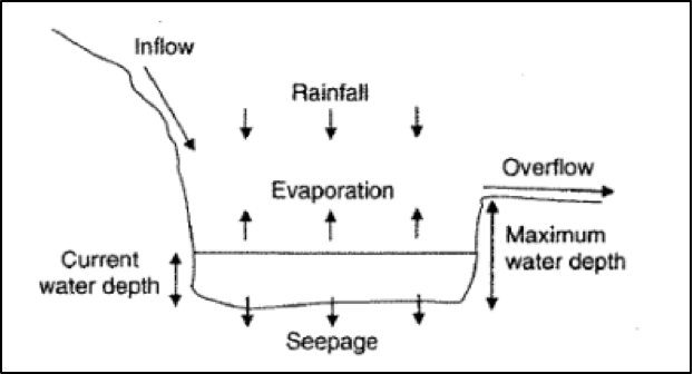
Figure 16: Conceptual model of lake water balance.
Surface waters can be either gaining (groundwater discharge to streams and lakes), losing (recharge of aquifers by streams and lakes), or through-flow systems (Winter et al. 1998). Based on the information you have, what type of lake (gaining, losing or through-flow) is the system shown in Figure 16? What other data might you want to measure to confirm this?
Simulating the system
Equation (11) is a differential equation, describing the rate of change of water level over time. We know that \(\frac{dh}{dt}\) is technically the instantaneous rate of change of lake water level. But calculus tells us that we can approximate \(\frac{dh}{dt}\) by calculating the change in water level over small increments of time, with the most accurate approximation using the smallest increments of time.
So we have an equation for the rate of change in lake water level (Equation (11)). But how do we calculate the lake level as a function of time, \(h(t)\)? That is, how do we solve this differential equation to calculate \(h\) for any given time? To do this we will use an iterative approach. Start with an initial lake level, \(h_{i}\), and then calculate the change in lake level over each small increment of time (in this case \(dt = 1\) year is fine), using the rates for each process. The water level at the next time-step is then calculated by summing the initial level and the calculated change; \(h_{i+1} = h_{i} + dh\). Would this step of going from \(\frac{dh}{dt}\) to \(h(t)\) be considered as differentiation or integration?.
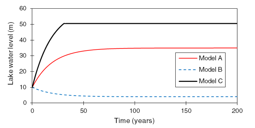
Figure 17: Simulated lake level under three different model scenarios (A, B and C).
| Parameter | Units | Model ? | Model ? | Model ? |
|---|---|---|---|---|
| \(r\) | m yr-1 | 1.00 | 1.50 | 1.00 |
| \(i\) | m yr-1 | 0.20 | 1.60 | 0.80 |
| \(e\) | m yr-1 | 1.00 | 0.05 | 0.05 |
| \(k\) | yr-1 | 0.05 | 0.05 | 0.05 |
| \(h_{\text{max}}\) | m | 50.00 | 50.00 | 50.00 |
Transient simulation
In the above simulations all model parameters are constant throughout the time period of the simulation, so that the results tell us what the “steady state” water level in the lake would be given those inputs and outputs. Let’s now see what happens if we have a time-varying (i.e. transient) input, we can call this Model D.
Let’s say that rainfall varies on decadal timescales, with wet (\(r\) = 1.5 m yr-1) and dry (\(r\) = 0.5 m yr-1) phases that alternate every 25 years. Start with a wet period and simulate water levels over 200 years using this transient rainfall distribution. Plot this new scenario on a chart along with the basecase. How do they compare? Does the lake ever overflow in this transient scenario?
If the lake is approximately circular, with a diameter of 50 m, what is the surface area of the lake? (hint: assume that the sides are steep so that lake surface area is independent of water level height). Based on this surface area, calculate the total volumes of seepage from the lakebed under these two scenarios (the basecase [Model A] and the transient model [Model D]). How do they compare, what is the effect of the transient rainfall input on the total volume of seepage? What does this tell you about the value of transient simulations vs steady state simulations?
Rates of change
Now let’s look at the rate of change in lake level under each of these modelling scenarios. Plot \(\frac{dh}{dt}\) vs time for each model (hint: remember that this is just the change in water level over time). How does this plot of \(\frac{dh}{dt}\) vs time relate to Figure 17? How long does it take for each model to reach “steady state?” How does the time it takes to reach steady state change if we used a different initial water level in our simulations?
Now have a go at making your own rainfall boundary condition. You may choose to base it on a probability distribution, or a have it randomly varying through time. Plot both lake water level and \(\frac{dh}{dt}\) vs time for your chosen rainfall distribution. How does this compare to the previous results?