Exercise 6 - Assessing impacts of environmental flows
Learning Objectives
At the completion of this exercise learners will be able to:
Describe the nature and importance of environmental flows
Predict the response of a wetland system to changes in flow regime
What are environmental flows?
Lakes, rivers and estuaries are adapted to receive water based on the natural hydrological condition, but often water is required upstream for other purposes. An environmental flow is water that is provided to the environment to maintain its health and natural diversity. In any river system, water and flows are needed in rivers to maintain:
Physical integrity of the river channel and floodplains (e.g., movement of sediment and maintenance of habitat)
Species and biological communities
Ecological processes (eg. nutrient, carbon, energy flow)
Ecosystem services:
- Flood attenuation
- Water purification
- Fish production
When we talk about river flows, from an eco-hydrology point of view, we can categorise them as having specific flow “components.”
- Extreme low flows - reduced connectivity and limited species migration
- Low flows / base flows - maintain adequate habitat; drinking water for terrestrial animals; and soil moisture for plants
- High flow pulses - Support feeding and spawning activities of fish
- Small floods (2 – 10yr ARI) - enable migration to flood plains, wetlands, and other habitats that act as breeding grounds and provide resources to many species. Drive reproduction processes of riparian plants
- Large floods (>10yr ARI) – Can change the path of the river, form new habitat, and move sediment and plant matter, connect remote environments
In simple terms environmental flows are a provision of water to satisfy environmental requirements for ‘healthy’ (natural) function. Environmental flows are a form of river/wetland restoration. They are sometimes referred to as “e-flows.”
When allocating water we try to maintain a “realistic” flow hydrograph based on historical (reference) data. But how do we measure the success or failure? Buying e-water costs a lot of money and is a politically charged issue. So we need to know we are getting it right!
Ideally we use a “flow-response” model - a measure of what ecological benefit we will get from a certain flow regime. But this is easier said than done, and measuring benefits is an important area of research.
So we need to use indicators – “measures of response.” This can include things like:
- Vegetation
- Water Quality (WQ)
- Biodiversity – e.g., fish / macroinvertebrate trophic index
We then monitor/assess indicators and adjust environmental flow management regime … in an ideal world.
Classifying e-flow benefits: A case study in the Murray-Darling Basin
In the Murray-Darling Basin (MDB), a water market was established that allows for irrigation entitlements to be “traded”; e-water must be bought from the “water holder” (in this case that is the Commonwealth Environmental Water Holder, CEWH). The overall management plan for the MDB uses a thing called Sustainable Diversion Limits (SDL’s) where managers identify what is able to be taken from the river, and in converse, what the river needs to function normally. The Murray-Darling Basin Authority (MDBA) also has a program called “FLOW MER” - Measuring Evaluation Research to help them monitor the effectiveness of their environmental flow regime.
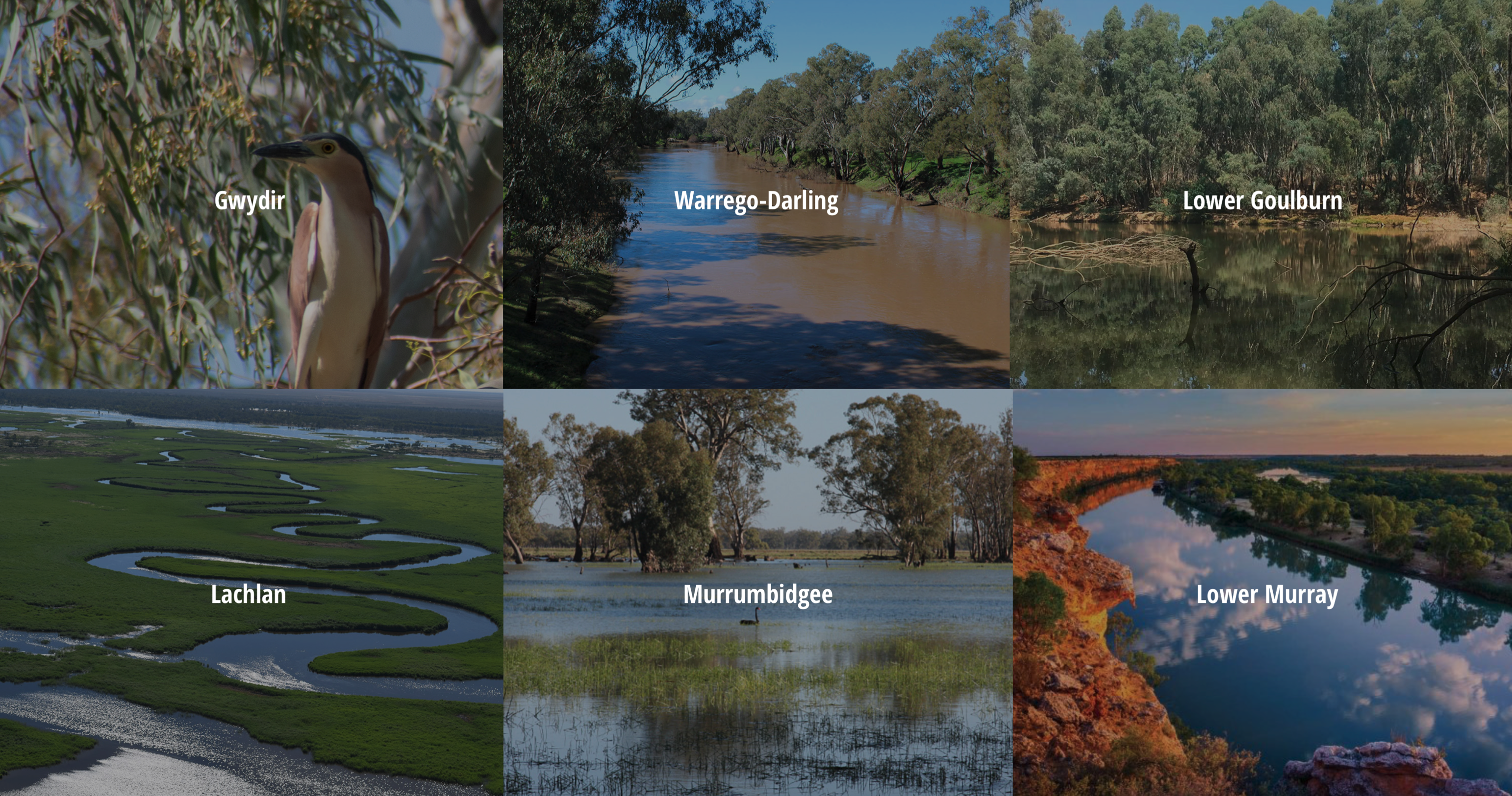
Figure 18: Focus study sites where environmental water delivery is assessed in the MDB. Visit: https://flow-mer.org.au
Take some time now to choose a selected MDBA focus site accessible from the above link. For your allocated/chosen focus region:
- Identify its location and key “values”
- Read the background and description of the approach to assessment of benefits
Review and be able to answer the following questions: - What are the expected stresses to be caused if natural water-flow regimes are lost? - List the current type of work being undertaken to assess how e-water is affecting the region - Describe the key findings / key learnings of the assessment that was undertaken at that site
Flow diversion case study : Robe Lakes
Figure 19: Explore the case study area with this interactive map.
We can further plan for e-water requirements to a critical system using scenario modelling, and as outlined above, the concept of “flow-response.” In this case we look at an example in South Australia where an assessment for water diversion is being undertaken, and we seek to look at what impact this might have on the salinity of a coastal lake. In other words, if we change the flow regime, what will the response be. In this case, salinity is an environmental indicator of ecological requirements.
Specifically in this example, we assess the impact of diverting water from “Drain L,” thereby reducing water to the Robe Lakes. Before we assess our diversion scenario, we must first analyse the historical flow data, to understand the historical flow regime.
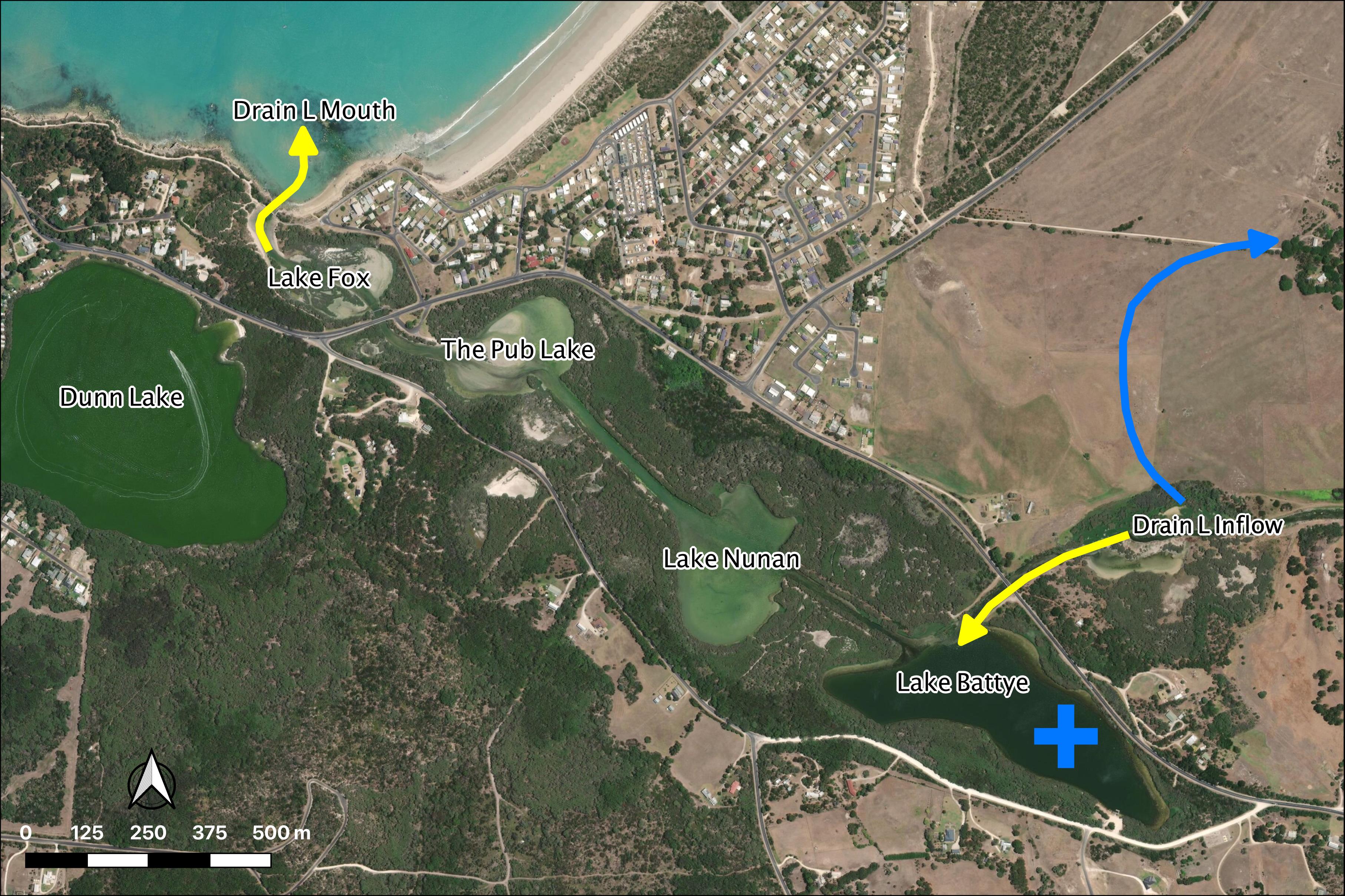
Figure 20: Drain L inflows (yellow arrow) will be diverted (blue arrow).
Module resources
Download the Excel spreadsheet for this module by clicking the download button in the tool bar .
Categorising flow data
You are given a time-series of daily river flow and need to assess how different diversion scenarios impact the freshwater flow delivery to a down stream estuary.
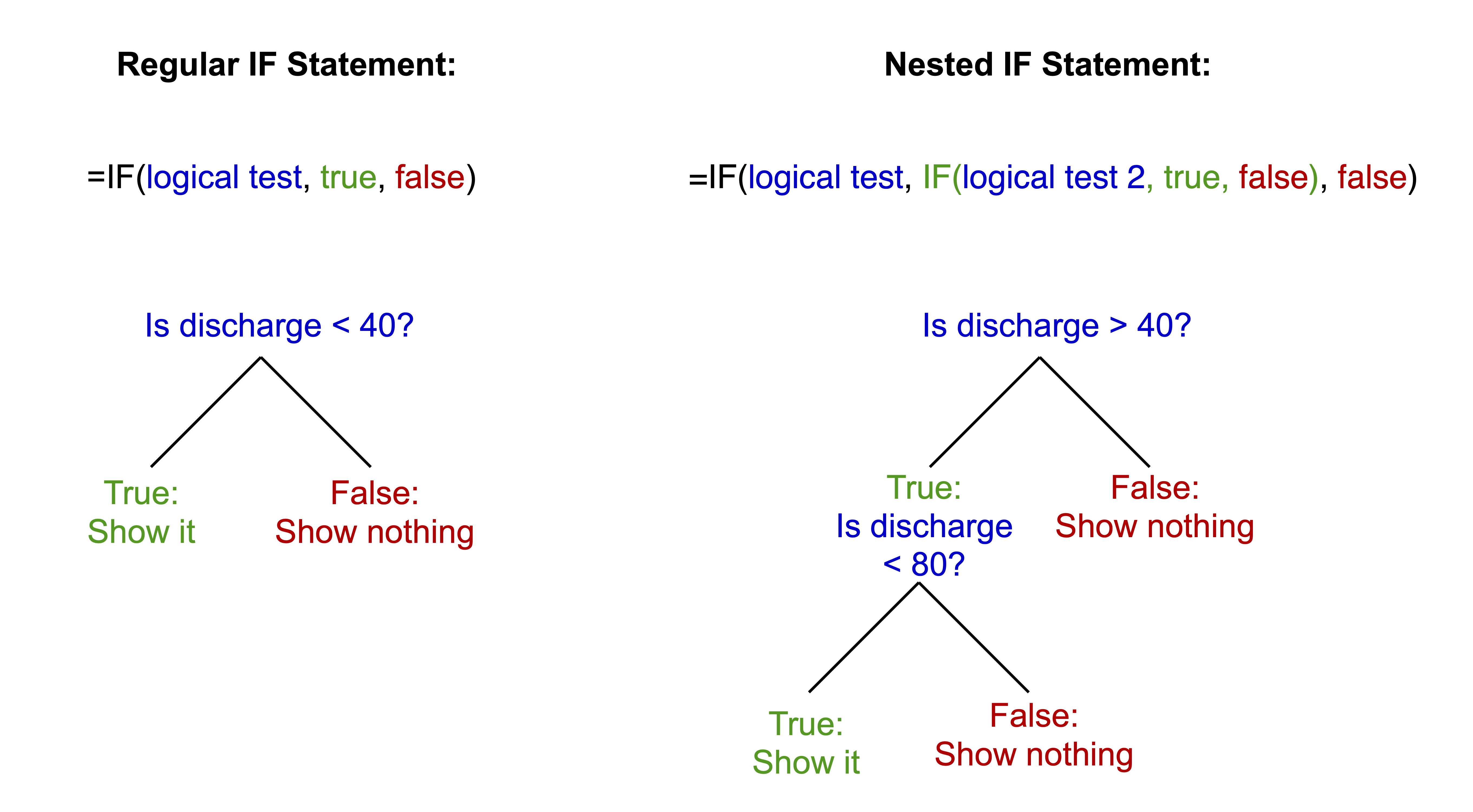
- For this flow time-series, calculate the volume of daily flow within the following bands 0-40; 40-80; 80-120; 120-200; 200-400; 400-1000; >1000
IF() statement in adjacent columns to partition flows
- For this flow time-series, calculate the number of days of daily flow within the above bands and work out annual average number of days
COUNT() to get the number of entries in the column
- Calculate the annual amount of flow in total and in each band
You may do the annual averaging manually or the pivot table method. For the pivot table method: Insert a new column B, Label it Year. Type the year number into the first cell, make sure it is formatted as a number.
Click two times on the little square in the corner of the box. This will fill down the page. Repeat this at each year change and you will have the year only information which you can then use to summarise data. As the original date has day numbers and decimal time each one is unique so you end up with a record for each day. This way you get a record for each year.
YEAR() to speed this step up
Highlight all the data. It must have headings for each column or it won’t work. Go to “Insert” then “Pivot Table.” Click OK as you want the default settings. Then you just fiddle until you get what you want. The following is an example:
Sort the years from highest to lowest total annual flow:
- Add a new column next to the flows indexing the years sequentially (i.e. 1, 2, 3…)
- Add a new column next to the indices calculating the probability of meeting the annual flow: \(P(Yri) = \frac{i}{\text{number of years}+1}\)
Flow diversion scenarios
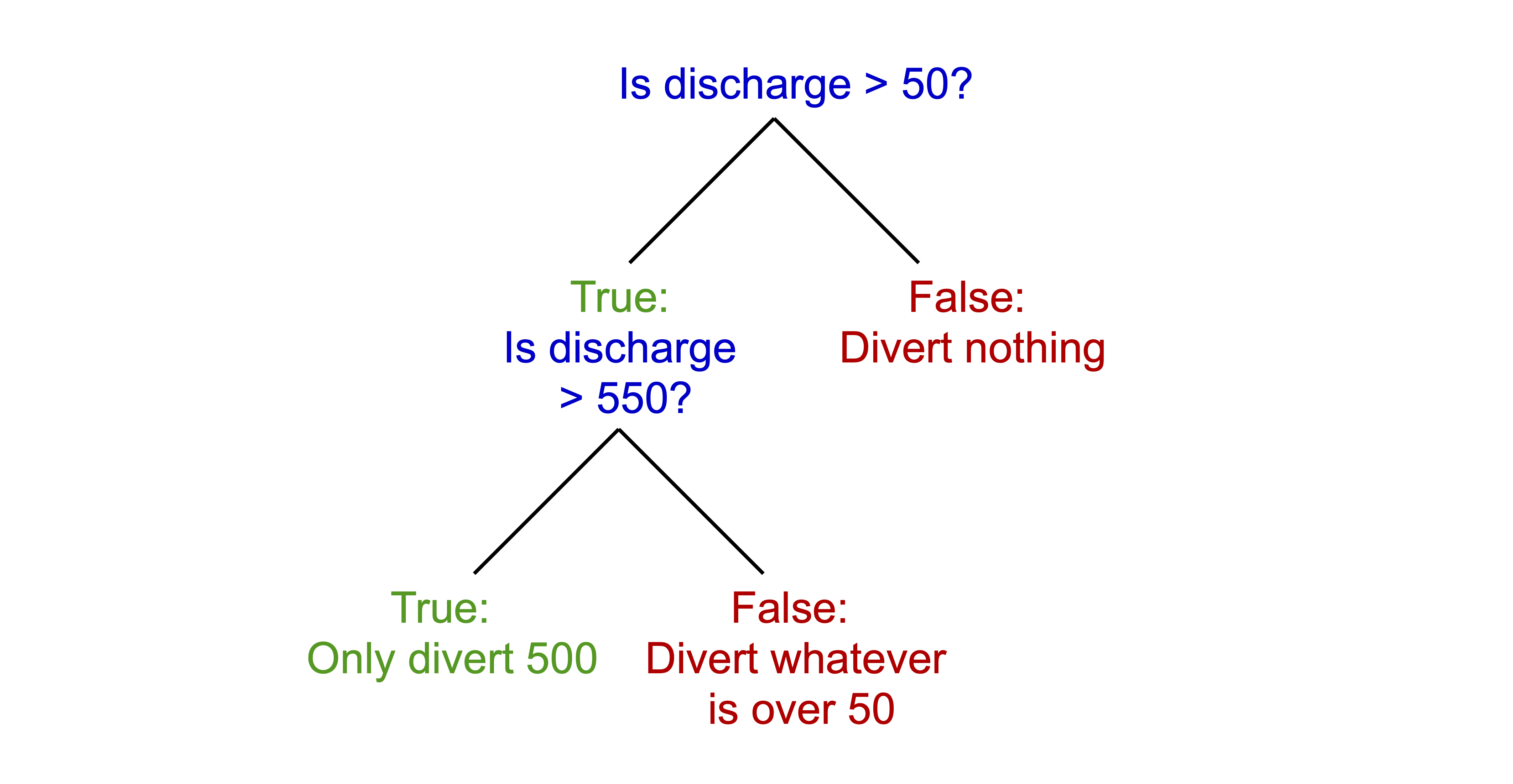
Assess the amount of water available for flow diversion for two scenarios by adding a new time-series column for each option:
- Water below 50 ML/day and above 550 ML/day is NOT diverted
- Water below 150 ML/day and above 1000 ML/day is NOT diverted
IF() that solves the following:
Add two new columns for each of the above to work out cumulative amount (running total) of diverted water
- \(\text{Cumulated Volume} = \text{Previous Cumulated Volume}+\text{Today's Diverted Discharge}\)
Assessing impacts on lake salinity
- Create a scatter plot of historical salinity (as EC) collected from the site marked in the map (+) vs daily discharge from the drain (see sheet: Estuary – Salinity).
- Fit a trendline to the data and display equation and R2 – this is a statistical model.
- In a new time-series column in the previous sheet, use the statistical model from above to predict a salinity time-series for the above station in the estuary under the two diversion scenarios compared to the base case.
Conclusions
In this exercise, we have explored the complexities of allocating water to the environment in a contested situation (i.e., where there are competing “customers” for the water resource). In particular, we can summarise environmental flows:
- appreciate that there is a potential conflict between e-flow vs irrigation allocation
- e-flow allocation is a river restoration and maintenance tool
- the array of benefits from e-water need to quantified and maybe site specific
- there is a need for identifying “Sustainable Diversion Limits” based on assessment of historical flow requirements.