Module 3: Climate Modelling
Energy Balance Models
Objectives
- To construct a simple energy balance climate model for the Earth in Excel
- To understand the role of greenhouse gases, and incorporate them into an energy balance climate model
Module resources
Download the Excel spreadsheet for this module by clicking the download button in the .
Case Study 1: A “Zero-Dimensional” Energy Balance Model
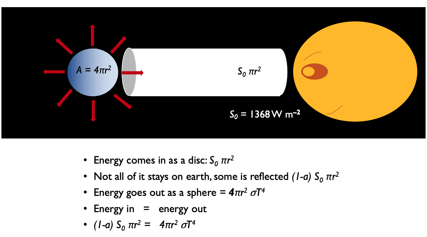
Here, we assume that the Earth is a sphere with uniform surface and no differences with latitude and longitude (i.e. everything receives the same amount of solar energy). We also assume that there is a balance, or equilibrium, between incoming short wavelength solar radiation absorbed by the ground and outgoing long wavelength radiation emitted by the ground. To simplify the model further, we assume the Earth emits outgoing (longwave) radiation like a “blackbody”, i.e. it is a perfectly efficient radiator - it gives off the maximum amount of radiation that an object of its temperature can emit.
Outgoing Radiation
The rate of the outgoing radiant energy (Joules per second = Watts) from a blackbody is given by the Stefan-Boltzmann equation:
where, \(\sigma\) = Stefan-Boltzmann constant (5.67x10⁻⁸), and \(T\) = Temperature (in degrees Kelvin).
However, for the Earth, this is being emitted over the full surface area of the Earth:
where, \(r\) = Radius of the Earth (in m).
Incoming Radiation
The energy absorbed by the earth is given by the amount of incoming solar radiation which is not reflected due to albedo. However, we have to take into account that solar energy is striking the Earth as a parallel beam of circular cross-section. So this incoming beam of radiation hits only a single “disc” of the Earth’s surface at any one time. This area has a surface area \(\pi r^{2}\).
where, \(S\) = incoming solar radiation: the “solar constant” (1367 W/m2) .
Exercises
Using the concept of an energy balance (i.e. energy in = energy out), rearrange the equations to find the Earth’s temperature, \(T\).
In Excel, construct a simple spreadsheet and fill in the blank cells of Table 1 to calculate the mean temperature of the Earth using the equation from Q1, assuming an albedo of 0.33 (including in °C and °F):
- The current mean temperature of the Earth is 288K (15°C). Does this simple model over or under predict the Earth’s temperature? What important factor is missing from this model?
| Parameter | Value | Units |
|---|---|---|
| Solar constant | 1367 | W/m2 |
| Albedo | 0.33 | No Units |
| Stefan-Boltzmann constant | 5.67e-08 | No Units |
| Mean temperature of Earth | K | |
| Mean temperature of Earth | °C | |
| Mean temperature of Earth | °F |
Remember: \(K = °C + 273.2\) and \(°F = 1.8°C + 32\)
- Test the sensitivity of this model to the choice of albedo. Using values from 0.3 to 0.7 in Table 2, calculate and plot T (°C)
| Albedo | Solar constant | Stefan-Boltzmann constant | \(T\) (K) | \(T\) (˚C) |
|---|---|---|---|---|
| 0.3 | 1367 | 5.67e-08 | ||
| 0.4 | 1367 | 5.67e-08 | ||
| 0.5 | 1367 | 5.67e-08 | ||
| 0.6 | 1367 | 5.67e-08 | ||
| 0.7 | 1367 | 5.67e-08 |
Case Study 2: A “Quick Fix”
To try to reduce the error in the model estimates of Earth’s temperature, we can “parameterise” the model using observed or experimentally derived relationships between outgoing radiation and temperature. One such example is:
Where, \(x = 204\) W/m2, and \(y = 2.17\) W/m2/°C.
This gets inputted into the energy balance equation (energy in = energy out) to give:
Exercises
Solve the above equation for \(T\) (note, this time, \(T\) is in CELSIUS!)
Set up a spreadsheet to estimate \(T\) for a range of albedo values. Different amounts of glacial ice cover on the Earth could produce albedos from 0.3 for minimal ice to 0.7 for a complete ice cover (this might seem unrealistic, but geologists have recently found evidence to suggest that the Earth was completely ice-covered during Neoproterozoic time 700 million years ago – a “snowball Earth”!)
- Are your results reasonably close for the present-day Earth mean temperature? What is the sensitivity of this model to small changes in albedo?
| Albedo | x | y | \(T\) (˚C) |
|---|---|---|---|
| 0.3 | 204 | 2.17 | |
| 0.4 | 204 | 2.17 | |
| 0.5 | 204 | 2.17 | |
| 0.6 | 204 | 2.17 | |
| 0.7 | 204 | 2.17 |
Case Study 3: Incorporating Greenhouse Gases
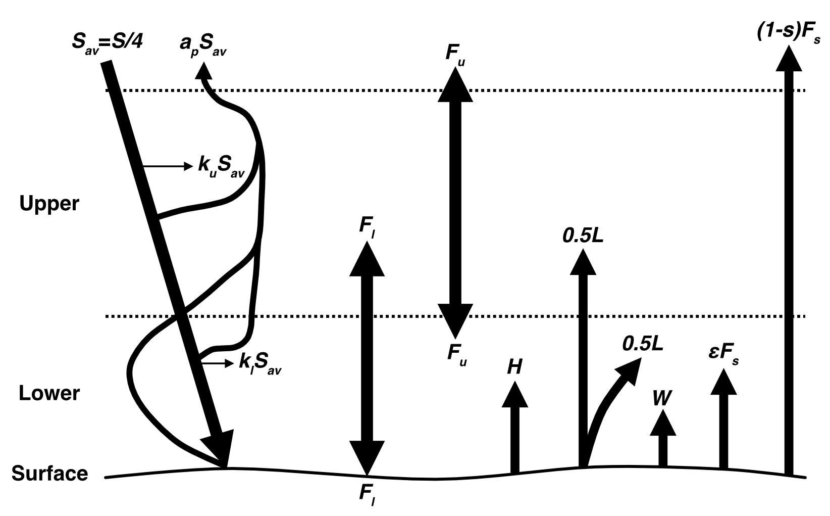
This model is a modification of the one described by Harte (1988). He showed that it is appropriate, based on the physics of radiation (as water is the major absolver of terrestrial radiation), to divide the Earth’s atmosphere into a lower layer (from the surface to 1.8km altitude, containing 20% of the air and 50% of the water vapour) and an upper layer (containing 80% of the air and 50% of the water vapour).
This time we require three energy-balance equations:
- For the Earth-atmosphere system as a whole;
- For the upper layer of the atmosphere;
- For the lower layer of the atmosphere.
In this model, all energy terms are expressed as long-term average fluxes, all temperatures are absolute. We assume that emissivity = 1 except at the surface, and (most importantly) that each of the three systems is in equilibrium.
| Parameter | Description | Value |
|---|---|---|
| \(S_{\text{av}}\) | Solar radiation intercepted by Earth (\(=\frac{S}{4}\) where \(S\) is the solar constant of 1370Wm-2) | 342.5 Wm-2 |
| \(W\) | Heat generated from nonrenewable energy sources (fossil fuels + nuclear) | 0.021 Wm-2 |
| \(L\) | Average latent heat flux from the surface | 80 Wm-2 |
| \(H\) | Average sensible heat flux at the surface | 17 Wm-2 |
| \(\sigma\) | Stefan-Boltzmann constant | 5.67 x10⁻⁸ Wm-2 deg-4 |
| \(a_{p}\) | Planetary albedo | 0.3 |
| \(k_{u}\) | Fraction of solar radiation absorbed in upper layer of atmosphere | 0.18 |
| \(k_{l}\) | Fraction of solar radiation absorbed in upper lower of atmosphere | 0.075 |
| \(\varepsilon\) | Emissivity (= 1 - reflectivity): the fraction of the infrared radiation emitted by the surface that is absorbed in the atmosphere and then re-emitted | 0.95 |
| \(F_{u}\) | Infrared flux from upper layer (use black-body equation) | \(\varepsilon \sigma T_{u}^{4}\) |
| \(F_{l}\) | Infrared flux from lower layer (use black-body equation) | \(\varepsilon \sigma T_{l}^{4}\) |
| \(F_{s}\) | Infrared flux from surface (use black-body equation) | \(\varepsilon \sigma T_{s}^{4}\) |
Exercise 1
Using the chart above, draw the model yourself by hand, incorporating all fluxes.
We can now formulate the three energy-balance equations needed:
Energy-balance for the Earth-atmosphere system as a whole:
Energy enters the Earth–atmosphere system from above at the rate \(S\) and from below at the rate \(W\) (heat generated from nonrenewable energy sources: nuclear and fossil fuels). Energy leaves these the system by three routes:
- Reflected solar radiation: \(a_{p}S_{av}\);
- Thermal radiation from the top of the atmosphere: \(\sigma T_{u}^{4}\); and
- The portion of thermal radiation from the surface that is not absorbed in the atmosphere: \((1 − \varepsilon)\sigma T_{s}^{4}\).
Here:
- \(\varepsilon\) is the fraction of surface radiation absorbed in the atmosphere (emissivity),
- \(\sigma\) is the Stefan-Boltzmann constant, and,
- \(T_{u}\) is the surface temperature (absolute). Thus, the energy balance for the whole system is:
Energy-balance for the upper layer of the atmosphere:
The upper atmospheric layer absorbs a fraction, \(k_{u}\), of the solar radiation that strikes it and also receives:
- Energy radiated upward from the lower layer: \(\sigma T_{l}^{4}\), and,
- One-half of the latent heat that accompanies evaporation from the surface (because this layer holds one-half the atmospheric water vapour): \(0.5L\). The upper layer loses energy by thermal radiation upward to outer space and downward to the lower layer. Thus, the energy balance for the upper layer is:
Energy-balance for the lower layer of the atmosphere:
Energy enters the lower atmospheric layer from above as absorption of a fraction, \(k_{l}\), of the solar radiation that enters it and as thermal radiation from the upper layer: \(\sigma T_{u}^{4}\). From below, energy enters from:
- The absorbed portion of thermal radiation from the surface: \(\varepsilon \sigma T_{s}^{4}\);
- One-half the latent-heat flux from the surface: \(0.5L\);
- The sensible-heat flux from the surface, \(H\); and
- The anthropogenic heat flux: \(W\).
Energy is lost from this layer by upward and downward radiation. The energy balance for the lower layer is therefore:
Exercise 2
Solve these equations to find a formula for surface temperature \(T_{s}\):
Equations (14) to (16) are a system of three equations in three unknowns: the temperatures \(T_{l}\), \(T_{u}\), and \(T_{s}\). The other quantities are parameters whose values must be given. The values of temperatures can be found via the following steps:
- Rearrange Equation (14) for \(\sigma T_{u}^{4}\) in terms of \(T_{s}\) and parameters.
- Rearrange Equation (15) for \(\sigma T_{l}^{4}\) in terms of \(T_{u}\) and parameters.
- Substitute the results of step 1 into the results of step 2 to give an equation for \(\sigma T_{l}^{4}\) in terms of \(T_{s}\) and parameters.
- Rearrange Equation (16) for \(\varepsilon\sigma T_{s}^{4}\) in terms \(T_{l}\), \(T_{u}\), and parameters.
- Put the results of steps 1 and 3 into the results of step 4 and simplify to give the equation for \(T_{s}\) as a function of parameters:
Using the values given in Table 4, what value do you derive for \(T_{s}\)?
How close is this to the actual value of 290K?
Exercise 3
Using Excel, test the sensitivity of this model to albedo. Compare your findings to those found in Case Study 1 (a plot of \(T_{s}\) for values of albedo between 0.3 and 0.7 might help here).
- For which model, and at what value of albedo, do you think the Earth would experience a strong positive feedback involving ice cover, albedo, and mean temperature, and therefore move rapidly toward “snowball Earth”? Could it ever be deglaciated?
Submission
Submit properly formatted graphs and tables of the following sections of the lab:
- Clear photograph or page scan of your hand drawn conceptual model of the Harte 1-D Energy Balance Model, including key explaining the terms.
- Clear photograph or page scan of your handwritten workings of the Harte Model calculations, with a clear answer of \(T_{s}\), the Earth’s temperature.
- Summary plot from Case Study 1, 2 & 3 assessing albedo and temperature of the three models, with a brief explanation of less than 150 words of which model you prefer.
- In 100 words or less, your answer to the Exercise 3 “snowball Earth” question.
These are to be uploaded as per the formatting specified in the Style Guide. Marks will be deducted for incorrect formatting.
References
Harte, John. 1988. Consider a Spherical Cow: A Course in Environmental Problem Solving. University Science Books.