Module 5a: Catchment Water Balance

Objectives

To understand a two-store catchment water balance model and implement within Excel. Using the supplied parameters and input data, run the model and plot changes in water stores and key hydrological fluxes.

Before you start

Listen to the water balance lecture
Be familiar with the connected bucket example (double buckets) in Excel

The Water Balance Approach

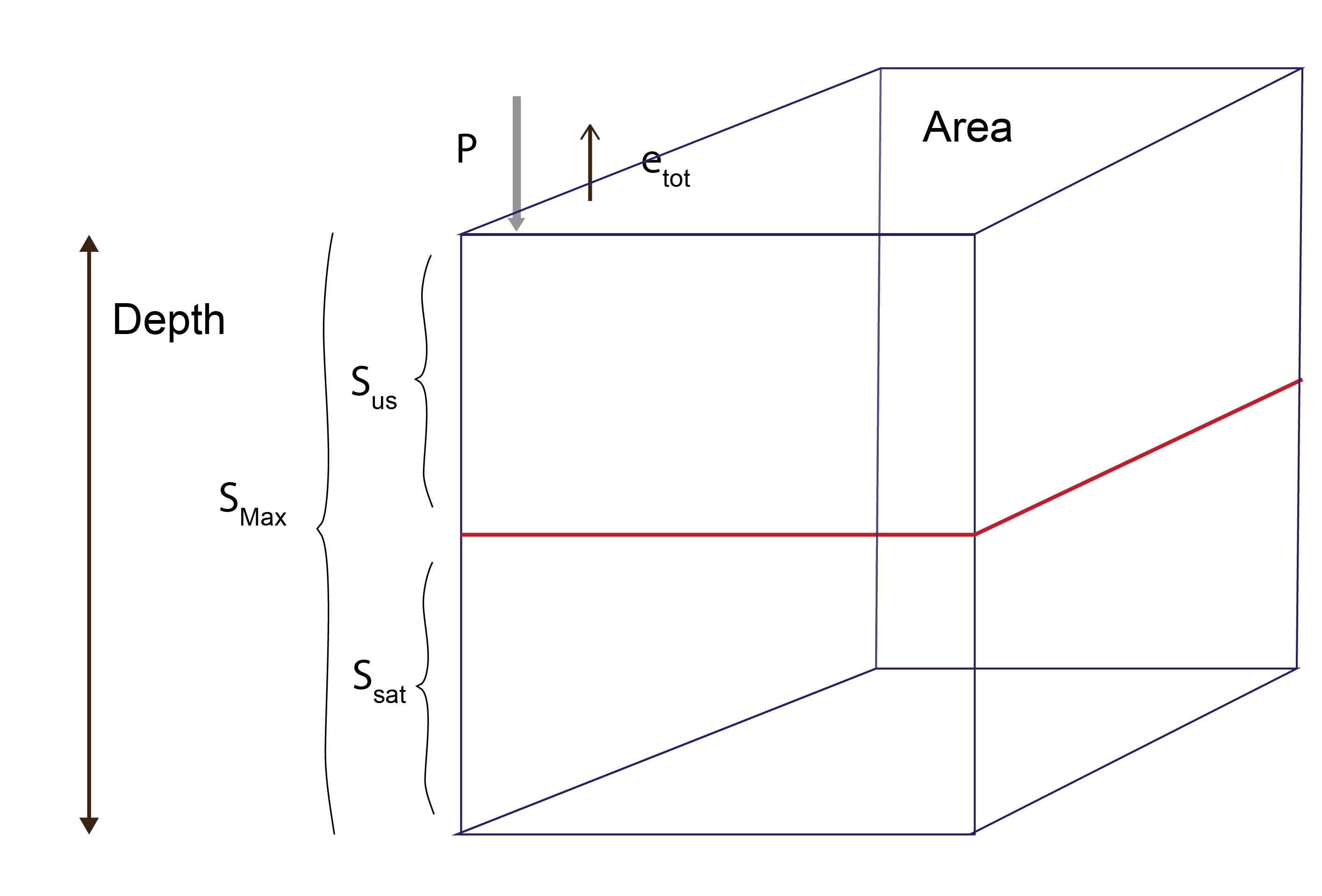
A water balance equation can be used to describe the flow of water in and out of a “system”. A system can be one of several hydrological domains depending on the context, such as a column of soil or a catchment basin. In the context of catchment, we assume the catchment area has a known ‘average’ depth, and the amount of soil is the catchment area multiplied by the depth. We treat this soil volume as our catchment ‘bucket’, and then estimate the inputs (rainfall) and outputs (evapotranspiration, runoff and baseflow).

Based on our understanding of soil physics, flow processes and transpiration, we can further partition water within the bucket into different sub-compartments. In this exercise we assume the catchment bucket can include a saturated and unsaturated layer, and even an optional deeper groundwater system.

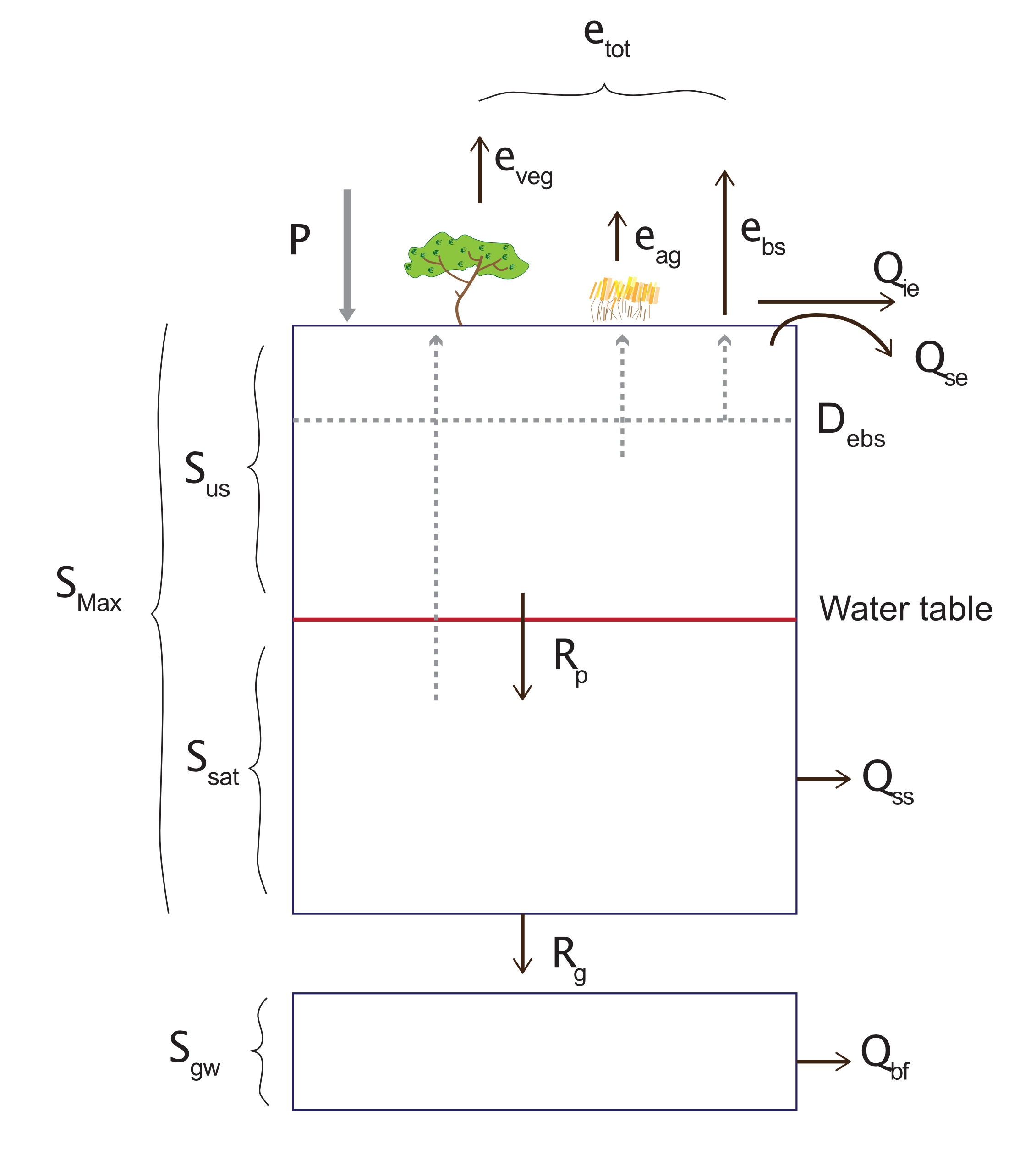
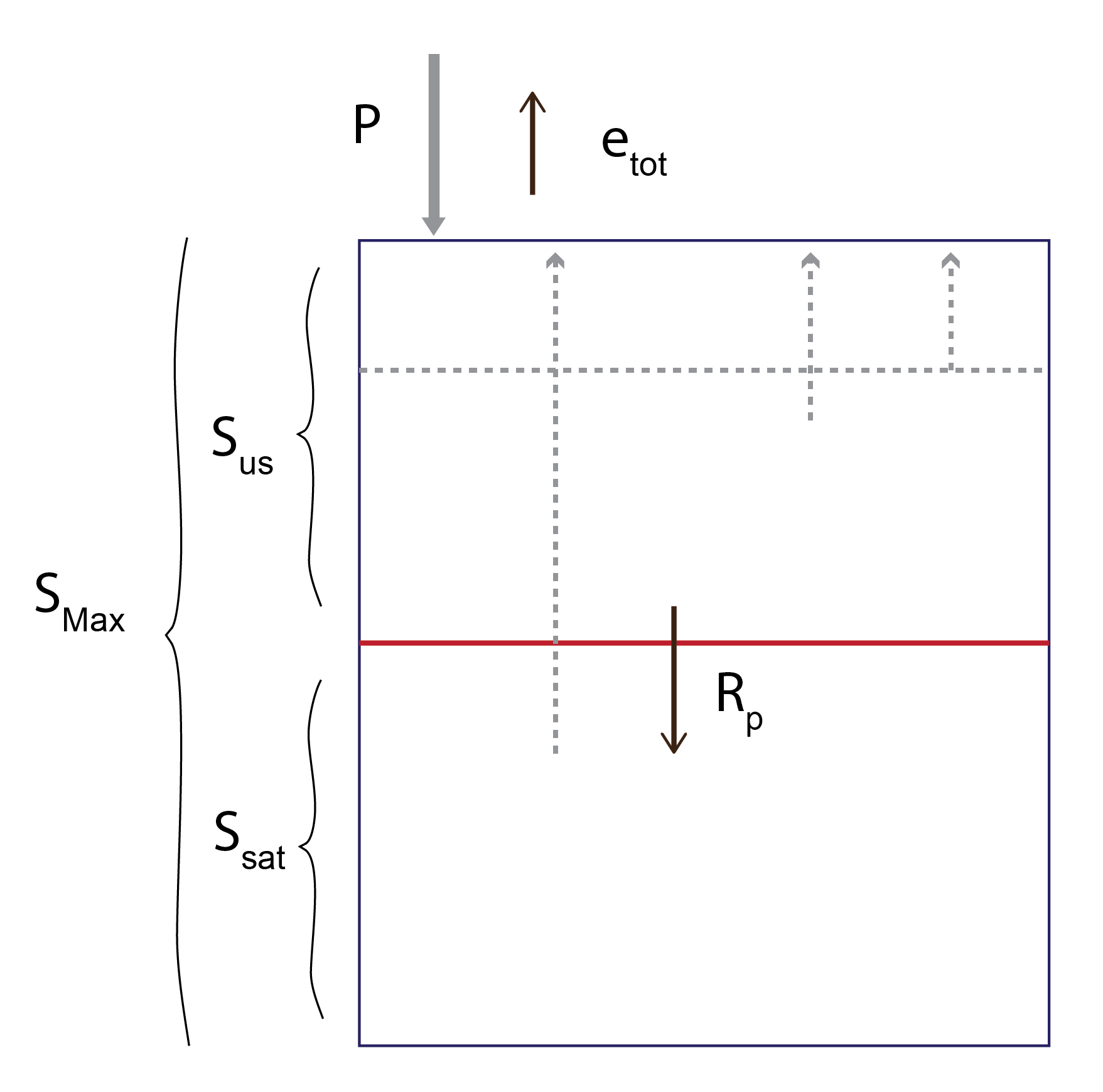
The water balance assumes an initial amount of water and then we sequentially estimate the fluxes of water as outlined below in the conceptual diagram.

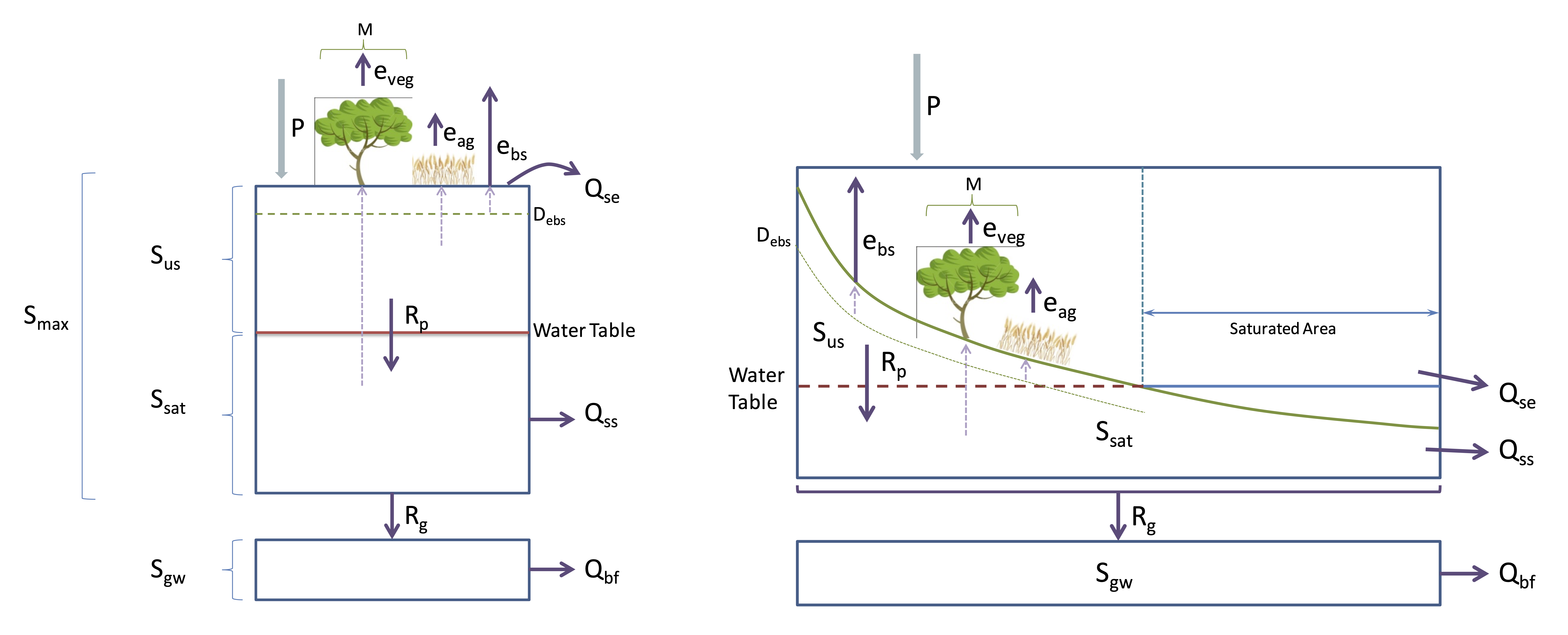
$Conceptual model schematic of the 0D ‘bucket’ by Yasmina Elshafei and Matthew Hipsey, adapted from Farmer et al. (2003). Note that $R_g$ and deep groundwater store $S_{gw}$ are depicted here as an optional extension and not included in the exercise.$

Figure 7: Conceptual model schematic of the 0D ‘bucket’ by Yasmina Elshafei and Matthew Hipsey, adapted from Farmer et al. (2003). Note that $R_g$ and deep groundwater store $S_{gw}$ are depicted here as an optional extension and not included in the exercise.

Module resources

Download the Excel spreadsheet for this module by clicking the download button in the tool bar .

Water Balance Model

Open the spreadsheet and familiarise yourself with the different sheets: CLIMATE, WATER BALANCE, PHOSPHOROUS, and SCENARIOS. Draw your own version of the diagram above, label all of the variables and note the storage, evaporation and flows.

1. Date

Have a quick look at the date.

In Excel, the date takes the first four columns of the WATER BALANCE sheet. Note that the dates increment with each row.

2. Climate

Navigate to the CLIMATE sheet. As boundary conditions, we have a precipitation dataset, and a function (Equation (32)) to simulate potential evaporation (Figure 8).

In Excel, the precipitation is in a column and has a value for every day. The potential evaporation is harder to get hold of. So we use a sine wave function, $sin()$, that takes an annual potential evaporation rate (e.g. 1.5m/yr) and makes a daily potential evaporation value that increases during summer and decrease in winter. Inspect, then copy this formula down the page.

Calculating Daily $e_p$ : Daily potential evaporation will be calculated using a sine wave, as follows:

\[\begin{equation} e_{p(\text{daily})}=\ \frac{e_{p(\text{annual})}}{365}\left[1+A\ \textbf{sin}\left\{B\left(m-1\right)+d\right\}+C\right]\ \tag{32} \end{equation}\]-23) \end{equation}

where, $A_{sin}$ is the height of the sine wave (i.e. maximum less minimum value), $B$ is the frequency of the sine wave, $C$ is the minimum $e_{p(\text{daily})}$ (i.e. in mid-winter), $d$ is the day of the month, and $m$ is the month number.

Figure 8: Potential evaporation sine wave function over time.

3. Storages

Start by copying your precipitation ($P$) and potential evaporation values from your CLIMATE sheet to your WATER BALANCE - 5a sheet. Next, type in the forumulas for storage using the equations given in the Equations section of this module. Take a look at $S_{tot}$ (Equation (37)) which is the total water in the two stores, $S_{sat}$ and $S_{us}$.

Note that there are two variables that have a prime ($\prime$) sign. These are interim storage values estimated so that we can use them for our IF statements to check for whether runoff or percolation should occur..

In Excel, there is an initial condition in a box given for you at time step 0. Your equations will start at time step 1. Your whole set of equations will not be finished until you have also completed the evaporation and flows, but you have to start somewhere.

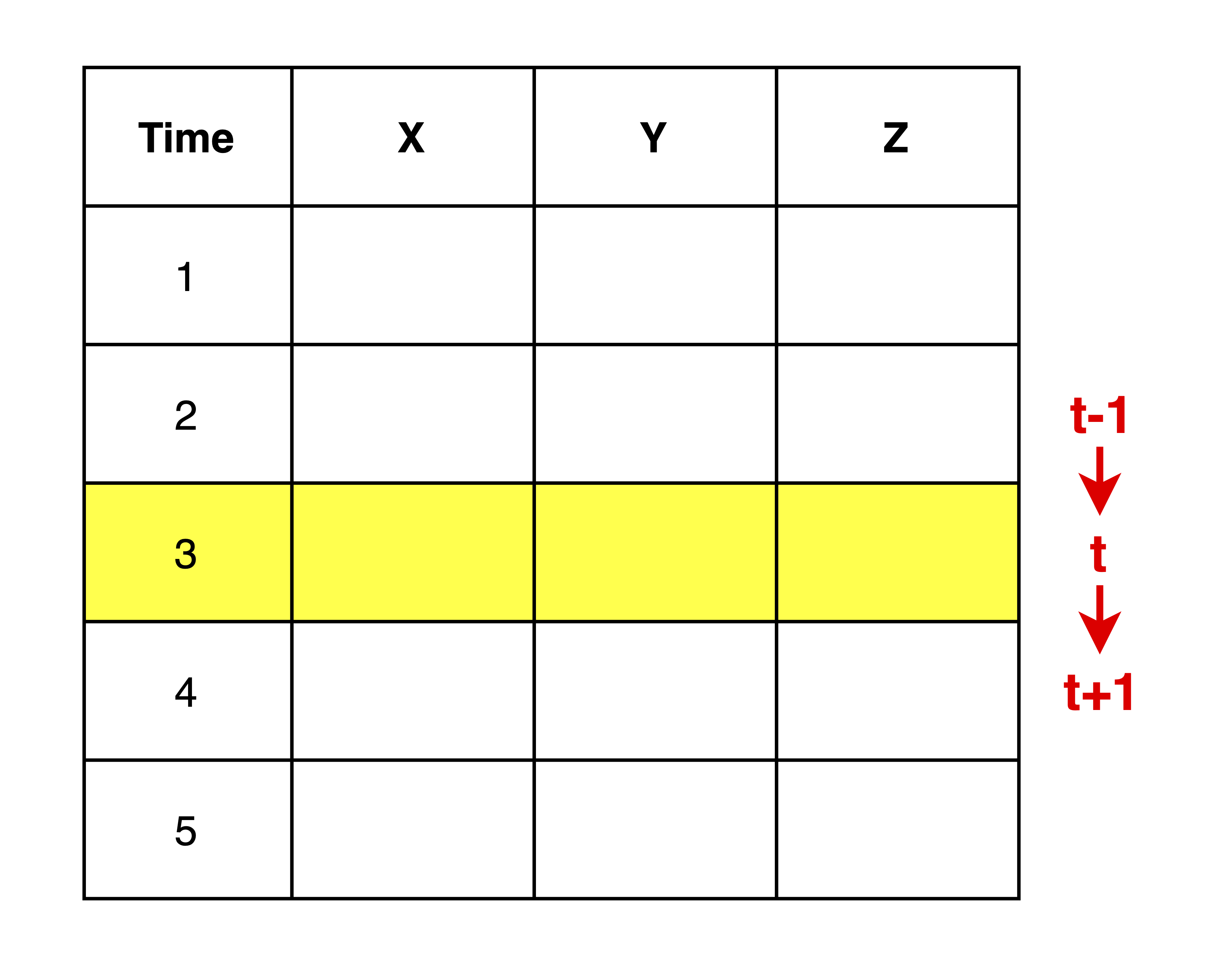
In Excel, the timestep advances as you go down the page. The notation $t$ could refer to any timestep, with $t-1$ simply being the timestep before $t$, and $t+1$ being the timestep after $t$.

If an equation is written entirely in terms of $t+1$ (e.g. $X^{t+1}= Y^{t+1}+Z^{t+1}$), it can be simplified to be written just in terms of $t$ (e.g. $X^{t}= Y^{t}+Z^{t}$). This is because $t$ is arbitrary and we’re just referring to the same timestep for the entire equation.

4. Actual evapotranspiration

Type in the evapotranspiration equations. Use the previous time step storage values to calculate these.

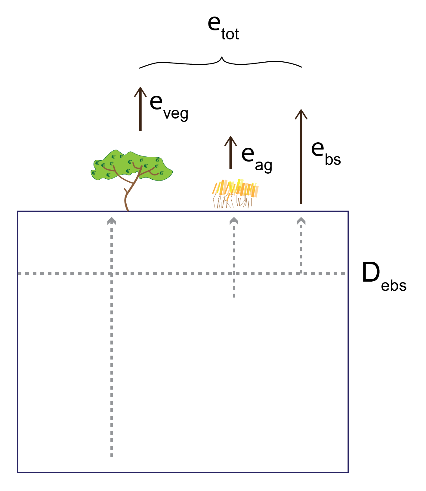
We are computing the water evaporating from trees tapping into groundwater ($e_v$) and from the unsaturated zone ($e_{bs}$ and $e_{ag}$)

5. Flows

Type in the flow equations, baseflow, infiltration excess runoff and runoff that occurs when the bucket is full.

6. Plots

When you have finished filling in all the columns, create some plots to explore the model. Consider a stacked-area plot of the two stores ($S_{sat}$ and $S_{us}$), and the evaporation components. Look at the fluxes like percolation and baseflow.

Play with the parameters and see what happens.

Notation

Forcing/Limiting Variables

$P$ = precipitation (m/d)

$e_p$ = potential evaporation (m/d)

$A_c$ = catchment area (m²)

Storage Variables

$S_{(t)}$ = total volume of water stored in catchment at time $t$ (m³)

$S_{max}$ = maximum storage capacity of bucket/ catchment (m³)

$S_{fc}$ = threshold storage i.e. storage at field capacity (m³)

$S_{us}$ = water storage in unsaturated zone (m³)

$S_{sat}$ = water storage in saturated zone (m³)

$S_{gw}$ = water storage in deep store (m³)

$f_c$ = threshold storage parameter i.e. 0 < $f_c$ < 1 (dimensionless)

$\theta_{fc}$ = field capacity (dimensionless)

$\theta_{pwp}$ = permanent wilting point (dimensionless)

$\varphi$ = porosity (dimensionless)

$D$ = soil depth from bottom (m)

$D_{ebs}$ = effective depth of influence from the bottom of the saturated zone for bare soil evaporation (m)

$D_{eag}$ = effective depth of influence from the bottom of the saturated zone for agricultural crop evaporation (m)

$S_{us(fc)}$ = current unsaturated zone field capacity (m³)

ET Variables/Fluxes

$e_t$ = total evapotranspiration at time $t$ (m/d)

$e_v$ = transpiration (m/d)

$e_{v(sat)}$, $e_{v(us)}$ = transpiration of deep rooted vegetation from saturated and unsaturated zone, respectively (m/d)

$e_{bs}$ = bare soil evaporation (m/d)

$e_{bs(sat)}$ , $e_{bs(us)}$ = bare soil evaporation from saturated and unsaturated zone, respectively (m/d)

$e_{ag}$ = agricultural crop evapotranspiration (m/d)

$LAI$ = leaf area index (dimensionless)

$M$ = % of catchment covered by deep rooted vegetation (dimensionless)

$C$ = % of catchment covered by shallow rooted agricultural crops (dimensionless)

$k_v$ = vegetation transpiration efficiency (dimensionless)

$K_s$ = saturated hydraulic conductivity (dimensionless)

$\alpha_{ebs}$ = bare soil evaporation scaling factor (dimensionless)

$\alpha_{eag}$ = agriculture evaporation scaling factor (dimensionless)

Flow Variables/Fluxes

$Q_t$ = total runoff at time $t$ (m/d)

$Q_{se}$ = saturation excess surface runoff (m/d)

$Q_{ss}$ = subsurface runoff (m/d)

$Q_{bf}$ = base flow (m/d)

$R_p$ = daily percolation $S_{us} \rightarrow S_{sat}$ (m/d)

$R_g$ = daily recharge $S_{sat} \rightarrow S_{gw}$ (m/d)

$\alpha$, $\beta$ = recession coefficients for subsurface flow from saturated zone

$\alpha_{bf}$, $\beta_{bf}$ = recession coefficients for subsurface flow from groundwater store

Equations

Maximum Storage Capacity of the Bucket/Catchment

Already completed in WATER BALANCE

\[\begin{equation} S_{max}=D\left(\varphi-\ \theta_{pwp}\right) A_c \tag{33} \end{equation}\]

The theoretical maximum storage capacity of the catchment is calculated by taking the difference between the porosity of the catchment soil (i.e. a measure of the total pore space in the soil, and hence, its ability to store water) and the permanent wilting point of the soil (the point at which volumetric water content is too low to be extracted from the soil by plants) and multiplying it by the volume of the catchment (i.e. surface area multiplied by the depth of the catchment). Note that $S_{max}$ is the sum of $S_{us}$ and $S_{sat}$, and does not include $S_{gw}$.

Note that ‘plant available water’ is the water content difference between field capacity and permanent wilting point of the soil at any given depth.

Threshold Storage

Already completed in WATER BALANCE

\[\begin{equation} f_c=\ \left(\frac{\theta_{fc}-\ \theta_{pwp}}{\varphi-\ \theta_{pwp}}\right) \tag{34} \end{equation}\]

Field capacity is the point at which all pore space small enough to retain water against the pull of gravity are filled (Brady and Weil, 1999). It is essentially the remaining water content of the soil after the removal of water by the downward forces of gravity over a daily time period. Field capacity therefore assumes that the water removed from the soil profile is only removed by gravity, not through plant suction or evaporation. The above formula calculates the threshold storage parameter as the proportion of ‘plant available water’ over storage capacity of the soil at any given depth.

\[\begin{equation} S_{fc}=\ S_{max} f_c \tag{35} \end{equation}\]

The volumetric water storage at field capacity is therefore the theoretical maximum storage capacity of the catchment multiplied (or limited by) the threshold storage parameter (which is ≤ 1).

Water Table Depth

The water table depth is calculated with the following equation:

\[\begin{equation} WT^{t}= \frac{S_{sat}^{t}}{A_{c}\varphi} \tag{36} \end{equation}\]

Water Balance

\[\begin{equation} S_{tot}^{t+1}= S_{tot}^{t}+(P^{t+1}- e_{tot}^{t+1})A_{c} - Q_{tot}^{t+1} \tag{37} \end{equation}\] \[\begin{equation} \color{grey}{S_{tot}^{t+1\prime}}= S_{tot}^{t}+ (P^{t+1}*A_{c}) \tag{38} \end{equation}\]

Water storage at any given time step, $t$, is calculated using the previous time step’s water storage as a starting point ($t$). Inflows and outflows of water from the system/ bucket are then incorporated to obtain the next consecutive value of $S$. Precipitation recorded in the current time step (inflow) is added to the initial storage value, whilst total evapotranspiration and total runoff (outflows) are both subtracted. Total water storage is made up of water stored in the saturated and unsaturated zones. Note that the initial value of $S_{tot}$ may be empirically determined or assumed to be a certain value. The initial value of $S_{sat}$ is taken to be $D$ less than the depth from the surface to the water table, which can be measured.

\[\begin{equation} S_{us}^{t+1}=\ \color{grey}{S_{tot}^{t+1^\prime}}-\ S_{sat}^{t+1} \tag{39} \end{equation}\] \[\begin{equation} S_{us(fc)}^{t+1}=\ f_c\left(S_{max}-\ S_{sat}^t\right) \tag{40} \end{equation}\]

Threshold storage in the unsaturated zone is simply the maximum potential storage capacity in the unsaturated zone multiplied (limited) by the threshold storage parameter.

\[\begin{equation} S_{us}^{t+1\prime}=\ S_{us}^{t} + P^{t+1} \times\ A_{c} \tag{41} \end{equation}\] \[\begin{equation} R_{p}^{t+1} = \left\{\begin{matrix} \color{grey}{S_{us}^{t+1^\prime}}-S_{us(fc)}^{t+1},\ \ &\color{grey}{S_{us}^{{t+1}^\prime}}>\ S_{us(fc)}^{t+1} \\ 0,\ \ &S_{us(fc)}^{t+1} \ge \color{grey}{S_{us}^{{t+1}^\prime}} \end{matrix}\right. \tag{42} \end{equation}\]

Equation (42) is an IF Statement.

The daily recharge rate from the unsaturated zone to the saturated zone is calculated as water storage in the unsaturated zone at the present time step, in addition to any new precipitation that has occurred, minus the threshold storage of the unsaturated zone (i.e. water which does not drain due to the downward forces of gravity alone). Recharge of this nature only occurs in the event that the combination of precipitation at the current time step, and water storage in the unsaturated zone, is greater than the threshold field capacity of the unsaturated zone.

\[\begin{equation} S_{sat}^{t+1}=\ S_{sat}^t+\ R_p^{t+1}-\ Q_{ss}^{t+1}-\ e_{v}^{t+1}A_{c} \tag{43} \end{equation}\]

Note the use of “$t+1$” on the Right Hand Side for $R$, $Q$ and $e$ will be on the same row since they are computed based on yesterday’s $S$.

The balance of volumetric water storage in the saturated zone is therefore calculated as the previous period’s storage plus any recharge from the unsaturated zone, minus outflows including recharge to groundwater, subsurface runoff, and total evapotranspiration (bare soil, deep rooted vegetation and agricultural crop) from the saturated zone.

Total Evapo-transpiration

\[\begin{equation} e_{tot}^t=\ e_v^t+\ e_{bs}^t+\ e_{ag}^t \tag{44} \end{equation}\]

Total evapotranspiration (ET) of the system is the sum of ET from deep rooted native vegetation, bare soil and agricultural crops in the catchment.

Native vegetation ET is calculated as follows.

Simple form:

\[\begin{equation} e_v^{t+1}= M \frac{S_{tot}^t}{S_{max}} k_v e_p^{t+1} \tag{45} \end{equation}\]

Agricultural/Shallow Root Crop Evapotranspiration

For evapotranspiration by agricultural crops, we make the assumption that they can draw water from the unsaturated zone only, thus:

\[\begin{equation} e_{ag}^{t+1}=C \alpha_{eag}[\frac{S_{us}^t}{S_{max}-S_{sat}^t}]e_{p}^{t+1} \tag{46} \end{equation}\]

Bare Soil Evaporation

\[\begin{equation} e_{bs}^{t+1} = \left\{\begin{matrix} (1-M-C)e_p^{t+1},\ \ &S_{sat}^t\geq\varphi D_{ebs} A_c \\ (1-M-C)\left[\frac{S_{us}^{t}}{S_{max} - S_{sat}^t}\right]e_p^{t+1},\ \ &S_{sat}^t<\varphi D_{ebs} A_c \end{matrix}\right. \tag{47} \end{equation}\]

This is an IF statement. In Excel split this equation up into the ‘TRUE’ and ‘FALSE’ columns.

Flows

\[\begin{equation} Q_{tot}^t = Q_{se}^t + Q_{ie}^t + Q_{ss}^t \tag{48} \end{equation}\]

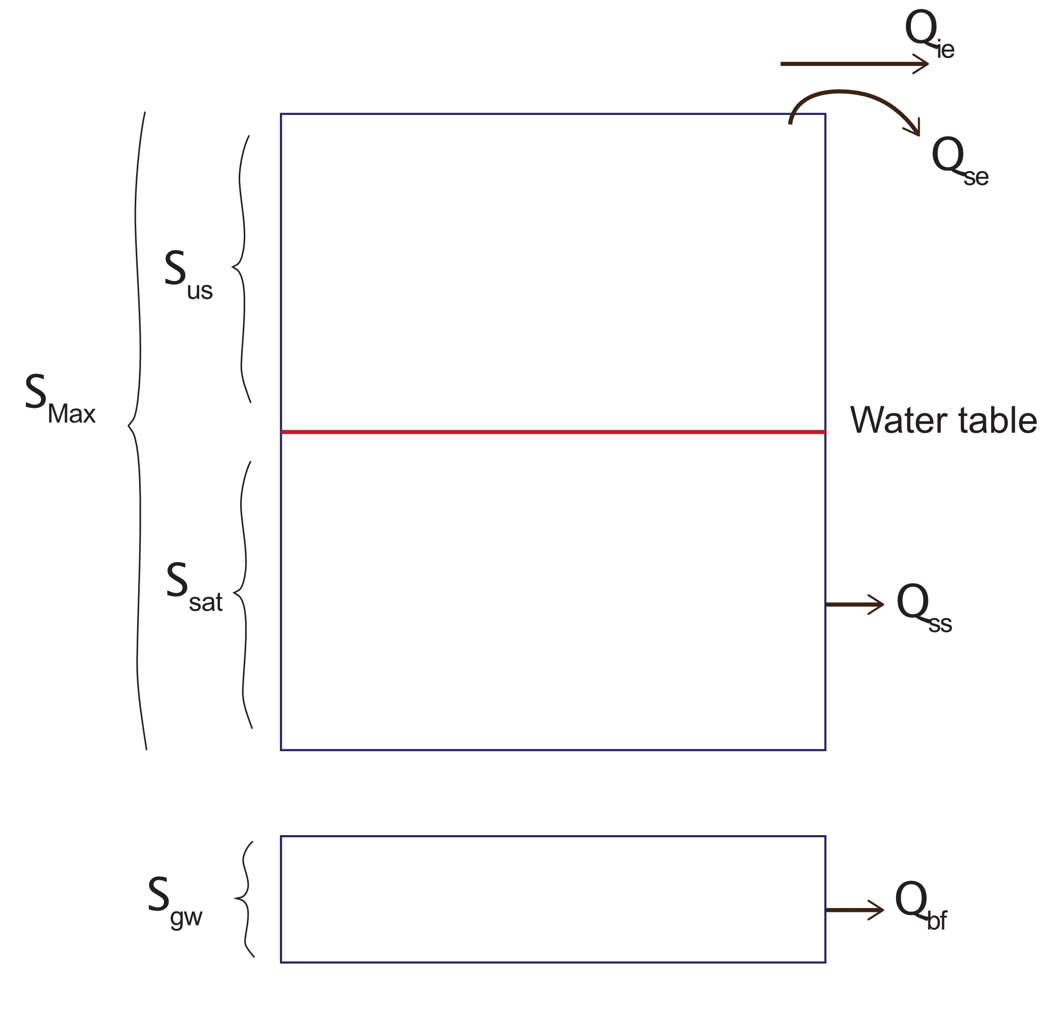
Total runoff of the system is the sum of saturation excess, infiltration excess, subsurface runoff, and (optional) base flow.

\[\begin{equation} Q_{se}^t = \left\{\begin{matrix} \color{grey}{{S}_{tot}^{t \prime}}-\ S_{max},\ \ &\color{grey}{{S}_{tot}^{t \prime}}>S_{max} \\ 0,\ \ &\color{grey}{{S}_{tot}^{t \prime}}\le S_{max} \end{matrix}\right. \tag{49} \end{equation}\]

Saturation excess is simply taken as being zero to the extent that water storage in the bucket/ catchment is less than maximum storage capacity. In the event that total water storage exceeds maximum capacity however, any excess is taken to be surface runoff.

\[\begin{equation} Q_{ie}^t = \left\{\begin{matrix} (P^t-I_{max})A_c,\ \ &{P^t}> I_{max} \\ 0,\ \ &{P^t}\le I_{max} \end{matrix}\right. \tag{50} \end{equation}\]

Subsurface flow:

\[\begin{equation} Q_{ss}^{t+1} = \left\{\begin{matrix} 0,\ \ &S_{sat}^{t}\le S_{usfc}^{t+1} \\ \alpha_{s}\frac{S_{sat}^t}{S_{max}}\ \ &S_{usfc}^{t+1} <\ S_{sat}^t \end{matrix}\right. \tag{51} \end{equation}\]

Subsurface runoff is taken to be zero in cases where the total water storage is less than field capacity threshold (i.e. thus will not drain due solely to the forces of gravity). In the event that total storage in the bucket/ catchment is greater than threshold storage and less than maximum storage capacity, subsurface runoff is taken as a nonlinear function using the excess above threshold storage and the assigned recession coefficients.

Submission

Submit properly formatted graphs and tables of the following sections of the lab:

Clear photograph or page scan of your hand drawn conceptual model of the Catchment system (may be combined with the 5b catchment model).
Stacked area plot of water storage over time
Plot of $Q_{ie}$ (infiltration excess runoff) and precipitation (on a secondary axis) over time
Plot of $Q_{ss}$(subsurface runoff) and precipitation (on a secondary axis) over time
Stacked area plot of $e_{v}$, $e_{bs}$, $e_{ag}$ (i.e. total evaporation) over time.

In less than 100 words write an answer to:

What is the general trend of rainfall over the long term?
What is the general trend of storage over the long term? Why does the storage vary over the short term?
Which flow mechanism contributes the most to the stream?
What is the dominant ET flux?

These are to be uploaded as per the formatting specified in the Style Guide. Marks will be deducted for incorrect formatting.