Module 5b: Land Use and Nutrient Management
Objectives
To setup a nutrient export model to compare the effect of best management practices (BMPs) on nutrient loads from a catchment with mixed land use.
Before you start
- Complete Module 5a
- Be familiar with the land use export model activity from lecture
- Review the flow concentration relationship document
- Review nutrient modelling lecture and be familiar with best management practices (BMPs)
Model Overview
Consider a catchment basin with with different types of land use.
The daily runoff/streamflow through the catchment, \(Q^t\) (m3/day), can be approximated based on the daily rainfall (\(R\)) - see the Water Balance model in Module 5a.
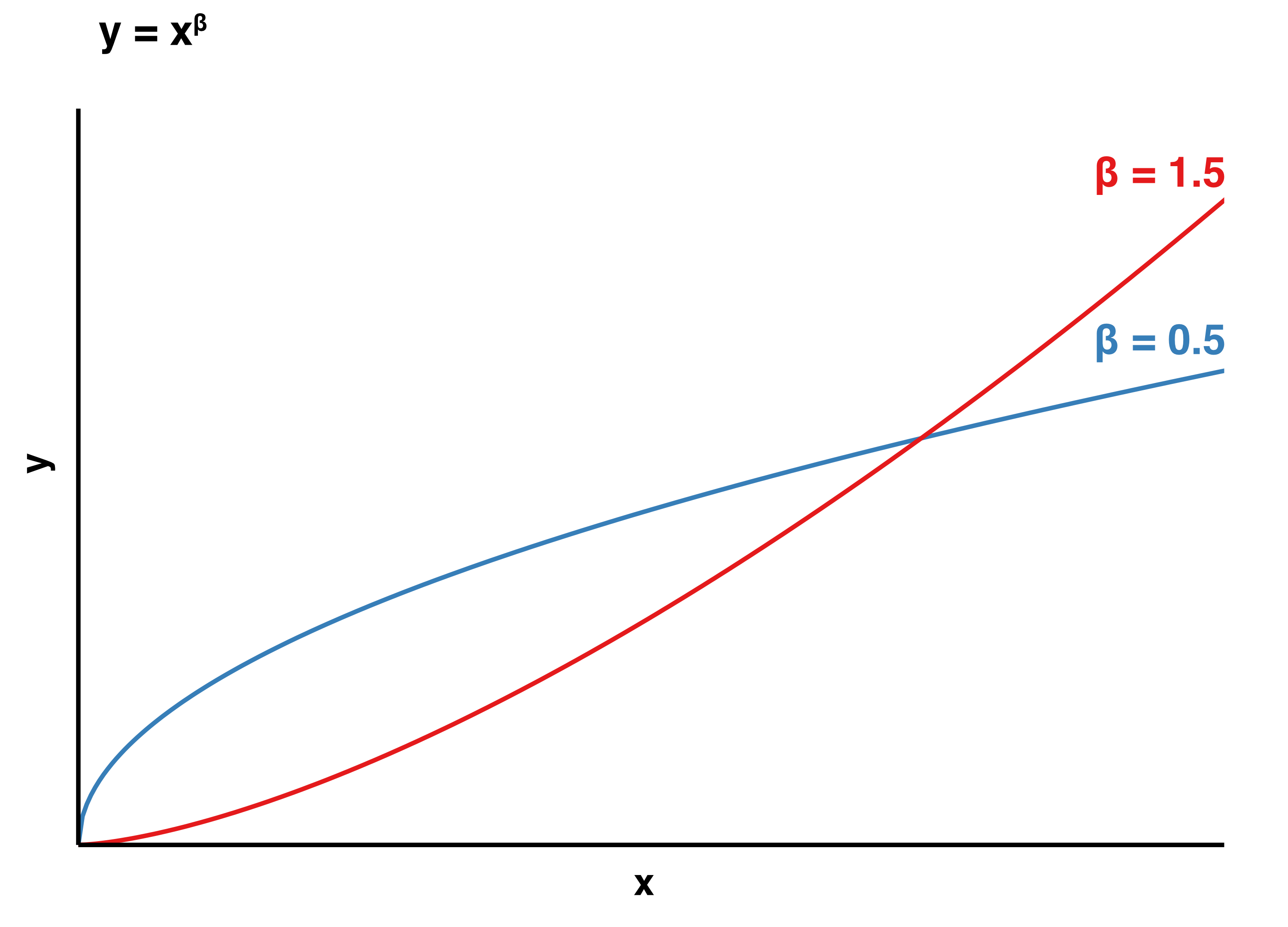
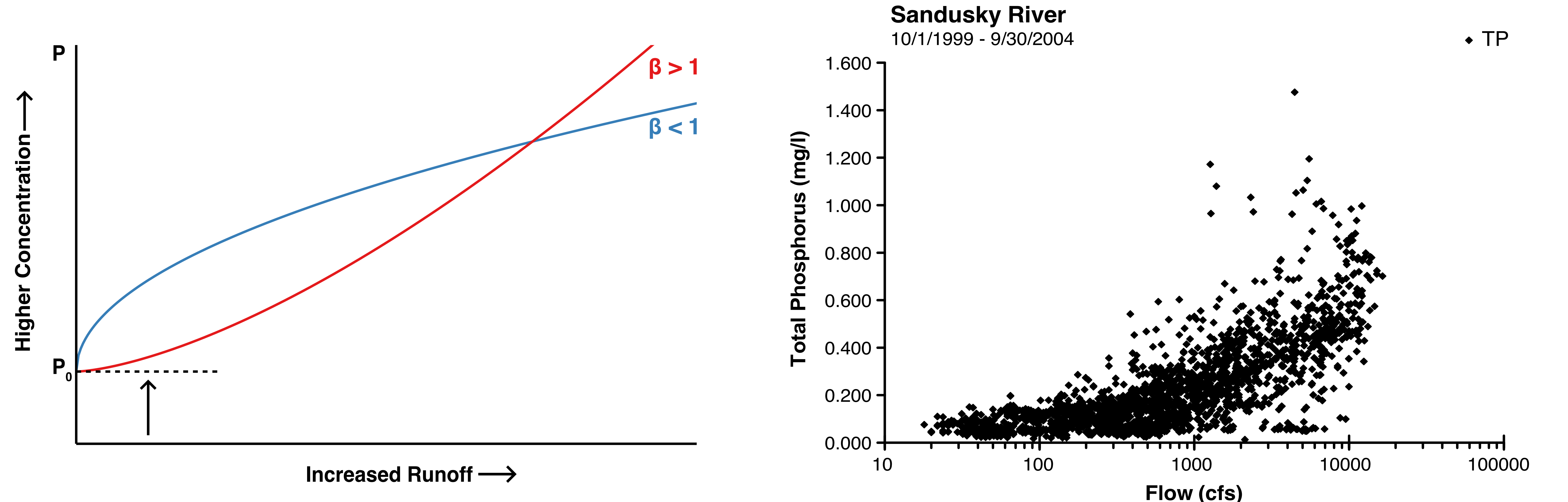
The phosphorus concentration in the water, \(P^{t}\) (g/m^3), depends on how much flow there is (i.e. more flow = more fertilizer leaching). To model this we use a simple power law to make a “flow-concentration relationship”, which is computed for each land-use (\(P\) is proportional to \(\alpha Q^{\beta}\)). If you’ve not seen a power law, sketch a graph of C (y-axis) vs Q (x-axis) for a value of \(\beta =1\). What happens if \(\beta =2\) or \(\beta =0.5\)?
This is averaged over the different land use fractions (denoted with the small \(p\) index), using the land-use fraction \(F_l\):
where alpha (\(\alpha\)) and beta (\(\beta\)) are variables that govern the stream \(P\) concentration (g/m3) as a function of area-averaged flow rate (\(Q/A\)) and they depend on the dominant land use (\(l\)). \(N_l\) is the number of land use classes being considered (4) and \(P_0\) is the background concentration (g/m3) for that sub-catchment (i.e. the value of PO4 when flow is low 0).
\(\color{#FF0000}{\alpha_{p} \left (\frac{Q}{A_{c}} \right )^{\beta_{p}}+P_{0}}\) is the flow dependent concentration (\(\color{#FF0000}{P}\)) of the p-th land use type.
\(P^{t} = \sum_{l=4}^{N_{p}} F_{p}\left (\color{#FF0000}{\alpha_{l} \left (\frac{Q^{t}}{A_{c}} \right )^{\beta_{l}}+P_{0}} \right )\) is a shorthand way of expressing: \(P^{t} = F_{1}\color{#FF0000}{P_{1}^{t}} + F_{2}\color{#FF0000}{P_{2}^{t}} + F_{3}\color{#FF0000}{P_{3}^{t}} + F_{4}\color{#FF0000}{P_{4}^{t}}\)The total \(P\) export load is \(P_{load}\) (g/day) and is the mass flux through the river (remember load = flow x concentration) :
Module Resources
The Excel spreadsheet for this module is part of the Module 5 download. Access using the download button in the tool bar .
Exercises
Building the model
- Draw by hand the conceptual model of this system.
- Confirm with the person beside you what index means (\(t\) and \(l\)).
- Set your modelled \(Q_{tot}\) to equal your \(Q_{tot}\) values in the WATER BALANCE - 5a sheet
Calibrating the model
Let’s make sure the model flows are realistic. Let’s compare our prediction with some observed data:
Create a regression plot of the observed \(Q_{tot}\) and your modelled \(Q_{tot}\)
Tailor this model to use the information as outlined in Table 6. Add a linear trendline, R2, and the line equation to the plot. Aim to achieve modelled flow values that closely match the observed \(Q_{tot}\)
| Parameters for catchment model: | Catchment value |
|---|---|
| Sub catchment area, \(A\) (km2) | 50 |
| Soil depth, \(D\) | 10 (m) |
| Baseflow coefficient, \(\alpha_s\) (range) | 5.0E3 to 5.0E4 |
| Field capacity, \(\theta_{fc}\) (range) | 0.08 to 0.15 |
| Infilt. capacity, \(I_{max}\) (range) | 0.01 to 0.3 |
| Deep rooted vegetation fraction, \(M\) (range) | 0.42 to 0.65 |
| Crop vegetation fraction, \(C\) (range) | 0.25 to 0.4 |
| Starting storage, \(S_{0}\) | 1.05E+08 |
| \(Ssat_{0}\) | 94500000.00 |
Manually adjust the catchment model parameters (see possible ranges in table above) until the model best matches the observed data - the observed flow data and water table data is in the CLIMATE sheet. This processed is called “calibration”.
Calculate phosphate concentrations
Now let’s work out the land-use specific stream \(P\) concentrations in the PHOSPHOROUS sheet:
- Predict the catchment river \(P\) concentrations and total export load, \(P_{load}\). The best way to do this is first predict the \(P\) concentration of each land-use class each as a column (i.e. Dairy \(P\) concentration, Wheat \(P\) concentration and so on), and then sum the 4 columns for \(P^t\) by factoring the (\(F_l\)) for each land-use.
| Parameters for P conc.: | \(\alpha\) (alpha) | \(\beta\) (beta) | land-use \(F_l\) |
|---|---|---|---|
| Landuse parameters: irrigated dairy (\(l\)=1) | 2.1 | 0.90 | 0.30 |
| Landuse parameters: wheat (\(l\)=2) | 1.2 | 0.45 | 0.10 |
| Landuse parameters: urban (\(l\)=3) | 1.9 | 0.80 | 0.15 |
| Landuse parameters: forest (\(l\)=4) | 0.5 | 1.20 | 0.45 |
Calculate phosphate export load
- Compute the \(P_{load}\) at the catchment outlet in kg/day. Also, work out the cumulative load (this will come in handy to coampre scenarios; we call it a mass curve)
Consider 2 management scenarios
Finally, let’s run 2 management scenarios:
8a) Scenario 1: If the total urban area expanded to 50% (0.5), how would this affect the overall \(P\) export?
8b) Scenario 2 If the irrigated dairy industry incorporated new phosphorus reduction technology, i.e. a best management practice (BMP) which leads to less \(P\) concentrations going from the farm to the stream. How would this affect the overall concentration in the water at the river basin outlet? The dairy concentration is now no more than 0.06 g m3.
Submission
Submit properly formatted graphs and tables of the following sections of the lab:
- Clear photograph or page scan of your hand drawn conceptual model of the Catchment system (may be combined with the 5a catchment model)
- Plot of calibration regression plot, including a trendline, equation and R2 value. Include in the caption what parameter values you gave the catchment.
- Plot of the cumulative phosphorous export of increased urbanisation (Scenario 1) and dairy management (Scenario 2) compared to the original conditions, over time.
- Plot of the concentration-flow relationship for the three scenarios of phosphorous concentration.
- Any other interesting plots you may like to create.
These are to be uploaded as per the formatting specified in the Style Guide. Marks will be deducted for incorrect formatting.