Module 6: River Pollution

Objectives

In this module you will setup an “advection-dispersion-reaction” equation for a river system to demonstrate the combination of temporal and spatial finite differencing, in one dimension.

Before you start

Review the mixing in the environment lecture
Undertake the lecture’s lake oxygen worked example

Advection-Dispersion Reaction

Mixing in environmental waters is described based on the currents and turbulence in the water - in simple terms we refer to these as advection and dispersion.

The advection-dispersion reaction equation for the concentration of a substance $C$, is defined as:

\[\begin{equation} \frac{\delta C}{\delta t} = D_{d}\frac{\delta^{2} C}{\delta x^{2}} - u \frac{\delta C}{\delta x} + S + R \tag{54} \end{equation}\]

where the left hand side (LHS) is the “unsteady” term ($C$ change in time), the first term on the right hand side (RHS) is the dispersion/mixing term, the second term on the RHS is the advection/movement term and $S$ is a source term, and $R$ is a reaction term. We use a partial deriviative (“curly $\delta$”) since $C$ is now varying in both space and time.

In this exercise we numerically solve the 1-dimensional, advective-dispersive transport of oxygen in a river. To solve this equation numerically, we must “discretise” the partial derivatives using finite difference methods, here done according to the FTCS scheme (refer to lecture!):

\[\begin{equation} \frac{C^{t+1}_{x}-C^{t}_{x}}{\Delta t}=D_{d} \frac{C_{x+1}^{t}-2C_{x}^{t}+C_{x-1}^{t}}{\Delta x^{2}}-u_{x}^{t} \frac{C_{x+1}^{t}-C_{x-1}^{t}}{2\Delta x}+R_{x}+S_{x} \tag{55} \end{equation}\]

Where the $t$ subscript is referring to timestep, and the $x$ subscript refers to the space increment/position. For the case of oxygen we assume that $R$ is accounting for oxygen input from the atmosphere and consumption by bacteria (called the Biochemical Oxygen Demand, BOD), then:

\[\begin{equation} R_x=k_a\left(C_a-C_x^t\right)-k_{BOD}C_x^t \tag{56} \end{equation}\]

Where the first term is atmospheric exchange ($k_a$ is the rate of re-aeration and $C_a$ is the saturation value of oxygen) and the second term is the bacterial consumption (described by $k_{BOD}$ which is in units of day^-1). We can solve for the forward timestep at any position along the river by computing:

\[\begin{equation} \small{C_{x}^{t+1}=\color{#898989}{C_{x}^{t}}+ \left [ \color{#3A88FE}{D_d \frac{C_{x+1}^{t}-2C_{x}^{t}+C_{x-1}^{t}}{\Delta x^{2}}}-\color{#FF2600}{u_{x}^{t} \frac{C_{x+1}^{t}-C_{x-1}^{t}}{2\Delta x}} + \color{#77BB41}{k_{a}(C_{a}-C_{x}^{t})}-\color{#B18CFE}{k_{BOD}C_{x}^t} \right ]\Delta t+\color{#D58400}{S_{x}}} \tag{57} \end{equation}\]

Previous $C$ concentration: $\color{#898989}{C_{x}^{t}}$

Diffusion: $\color{#3A88FE}{D_d \frac{C_{x+1}^{t}-2C_{x}^{t}+C_{x-1}^{t}}{\Delta x^{2}}}$

Advection: $\color{#FF2600}{u_{x}^{t} \frac{C_{x+1}^{t}-C_{x-1}^{t}}{2\Delta x}}$

Atmospherical exchange: $\color{#77BB41}{k_{a}(C_{a}-C_{x}^{t})}$

Biological O₂ demand: $\color{#B18CFE}{k_{BOD}C_{x}^{t}}$

O₂ source/sink: $\color{#D58400}{S_{x}}$

To solve this the user specifies the initial oxygen concentration ($C_0$), river velocity ($u$) as a function of distance, grid length ($L$), grid spacing ($\Delta x$), simulation period ($T$), time step ($\Delta t$). The calculation should then compute the change in oxygen as a function of distance and time.

Extra sources or sinks of oxygen can by added into the domain based on the $S$ term. We will first set up the model to have no $S$ inputs along the side of the river, but in the last task we add a low oxygen discharge somewhere along the river (ie. a pipe outflow).

Module Resources

Download the Excel spreadsheet and R files for this module by clicking the download button in the tool bar .

You can use either Excel or R for this module.

Exercises

Setting up the Model

Draw the schematic of the conceptual model by hand, showing the spatial discretisation, boundaries, sources, reactions, and a little animal swimming in the river.
Start with the provided spreadsheet or R script, and implement the above expression. Set up the spreadsheet to assume a river of length ($L$) ~5 km. You will need to select an $x$ increment ($\Delta x$).

In Excel, time is going down the rows and distance (space) is going along the columns.

Set the initial condition ($C_0$) row to be 10 mg O₂/L – i.e. the whole river starts at 10 mg/L in each cell.
Once you see the formula is working in the first time-step, then copy the formula along the length of the river. You will need to set a downstream boundary condition (at the the position where $x = L$, the last column). For this we will set a “zero-derivative” condition $– \frac{\delta C}{\delta x} = 0$. Therefore $C_n = C_{n-1}$, where $n$ is the last cell of the river length.
Copy the first time row down for all the time-steps (simulate several days in total).
Plot the oxygen concentration as a function of distance for several times during the simulation.

For Excel users, Set up conditional formatting to help visualise the concentration change through space and time

Modelling a Wastewater Plume

Implement at $x \approx 1500\text{m}$ a wastewater plume entering the river – do this by reducing the $C$ at the relevant $x$ cell by 3 mg/L (or less if the $C$ is already below 3). This is done by adding the extra “$S$” term of -3 to the appropriate $x$-cell formula, and copying the formula down through time. Plot and note how the oxygen recovers downstream of the low oxygen inflow plume.

To prevent negative O₂ concentration (in otherwords, we can’t take more than is available) we cap the solution to be greater than 0. Preventing negatives can be done as: =MAX(equation, 0 )

Advection and dispersion of O~2~ in a river of length $x$. Note, in this figure $W_c$ refers to our wastewater plume (click [here](https://hydrologie.org/BIB/Publ_UNESCO/SR_999_E_2005.pdf) for image source).

Figure 9: Advection and dispersion of O₂ in a river of length $x$. Note, in this figure $W_c$ refers to our wastewater plume (click here for image source).

The above example should show the low oxygen water diffusing into the river environment. The default velocity in this river was 0.2 m/s which is not very fast. Increase the velocity ($U$) in all cells to 1.2 m/s and see how the shape of the waste water plume changes. Now the advection term will be more significant, you should see the plume moving more strongly down stream.

Modelling an O₂ Drop

Change the upstream boundary concentration at $x = 0$, to include a sudden drop in oxygen for a period of 0.5 hour. Plot how this signal propagates through the river domain during and after the period where the upstream condition drops – can you see the low oxygen pulse moving through the river? How does this concentration profile vary if the diffusivity is different?

Modelling your own Scenario

Create your own environmental scenario using this model, make a brief description of it, calculate a result and if necessary, express the result with a figure.

If you see fluctuating negative and positive concentrations, you might have numerical instability. Adjust your $\Delta t$ or $\Delta x$.

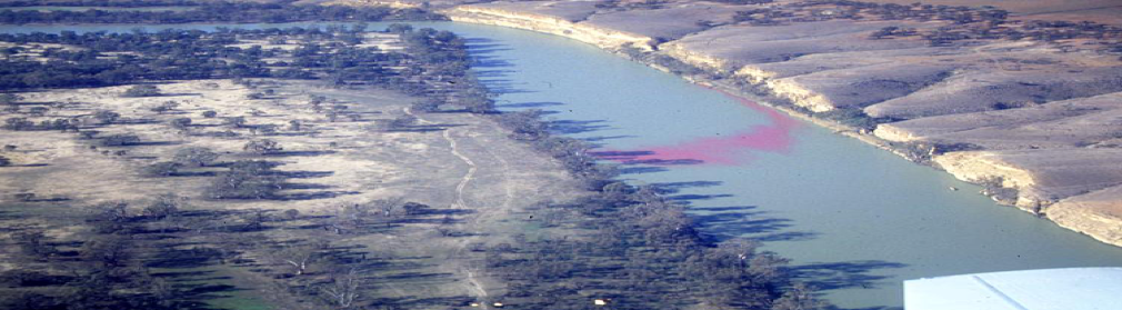
Figure 10: A plume of coloured dye dispersing through a river.

Submission

Submit properly formatted graphs and tables of the following sections of the lab:

Clear photograph or page scan of your hand drawn conceptual model of the river with all the oxygen transport processes labelled.
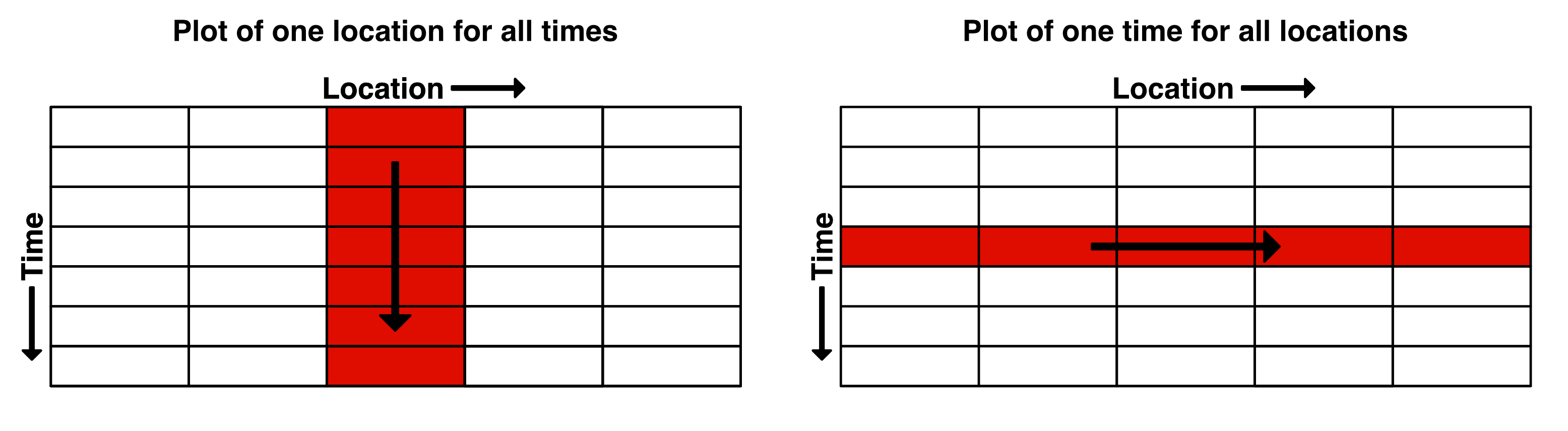
A plot of oxygen concentration at several times plotted for all distance of the river.
A plot of oxygen concentration at several points of the river plotted for all time.
A plot of the oxygen concentration with the upstream boundary drop at several points of the river plotted for all time.
A plot of the oxygen concentration with the wastewater plume at several times plotted for all distance of the river.

A plot of your own individual environmental scenario.
- Don’t plot too many lines – only several are necessary and use your judgement to select how many show the results well whilst the plot still clear and easy to understand.
- Make sure your axes are well labelled and clear to read. If abbreviating oxygen, include a subscript in O₂.

These are to be uploaded as per the formatting specified in the Style Guide. Marks will be deducted for incorrect formatting.