Module 4: Ocean Acidification

Objectives

• Calculate the carbonate species distribution given pH and CO₂ (gas)
• Build a double-log plot based on a range of pHs
• Calculate the pH change and CaCO₃ solubility given an increased atmospheric CO₂.
• Replot other published data for comparison with our data

Before you start

• Review slides

Overview

In this exercise, we create a simple model of the ocean, with a limited number of state variables. We examine the chemical interactions that result from atmospheric CO₂ gas dissolving in water, along with calcium salts in the ocean fed by erosion of minerals on the land. The key overall process is that dissolved CO₂ and Ca²⁺ are in equilibrium with solid CaCO₃ (limestone).

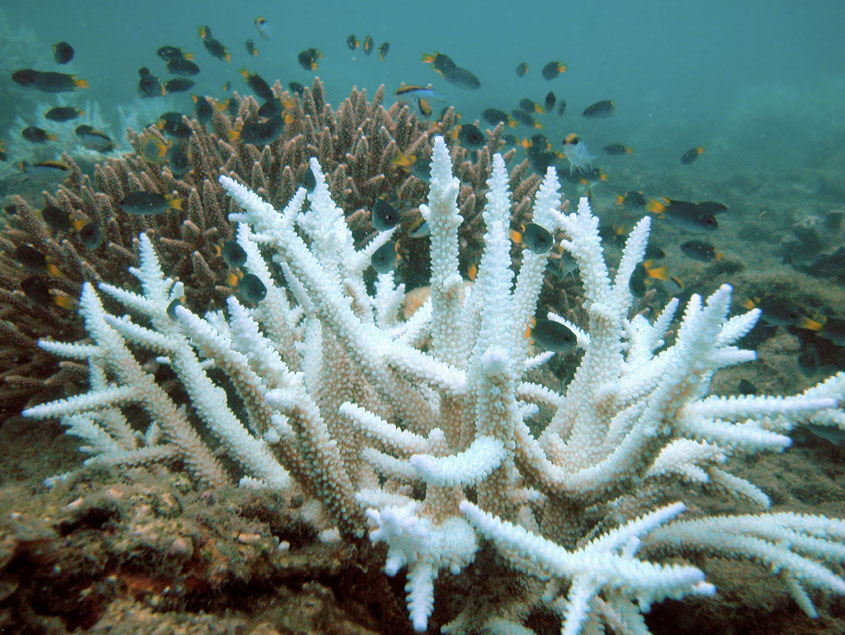
Figure 3: Bleached coral (foreground) and normal coral (background). CC BY 3.0, https://en.wikipedia.org/w/index.php?curid=32829631

The major variables are given in Table 5. Given any two of the variables on the left hand column, the other four can be calculated.

Table 5: Major variables

\(CO_{2 (\text{gas})}\)	\(CO_{2 (\text{dissolved})}\)
\(H^{+}\)	\(Ca^{2+}\)
\(HCO_{3}^{-}\)	\(OH^{-}\)
\(CO_{3}^{2-}\)	\(H_{2}CO_{3}\)
\(C_{T} \text{ (total dissolved inorganic carbon)}\)	\(H_{2}CO_{3}^{*}\)
\(\text{Alkalinity}\)

Module resources

Download the Excel spreadsheet and R files for this module by clicking the download button in the tool bar .

You can use either Excel or R for this module.

Exercise 1

In the first exercise, we set pH to be 8.3 and atmospheric CO₂ gas to be 3.5×10^-4 atmospheres, and calculate the other variables based on these two. CO₂ gas dissolves in water according to Equation (18). The dissolved CO₂ easily dissociates into carbonic acid according to Equation (19). For simplicity, we will go straight from atmospheric CO₂ to H₂CO₃*, which is the sum of dissolved CO₂ and carbonic acid, using Equation (20).

\[\begin{align*} {CO}_{2(\text{gas})}&\rightleftarrows{CO}_{2(\text{dissolved})} \tag{18} \\ {CO}_{2(\text{dissolved})}+H_2O&\rightleftarrows H_2{CO}_3 \tag{19} \\ {CO}_{2(\text{gas})}+H_2O&\rightleftarrows \color{#ED7D31}{H_2CO_3^\ast} \hspace{3em} K_{H} = 3.39×10^{-2} \tag{20} \\ \end{align*}\]

The carbonic acid dissociates into a hydrogen ion (H⁺, or proton) and a bicarbonate ion (HCO₃^-), according to Equation (21). The bicarbonate further dissociates into carbonate (CO₃^2-) and another hydrogen ion, as shown in Equation (22). The release of these two hydrogen ions is what creates the acidity of the ocean.

\[\begin{align*} \color{#ED7D31}{H_2CO_3^\ast} &\rightleftarrows \color{#00B050}{HCO_3^-}+\color{#FF0000}{H^+} \hspace{3em} K_{1} = 5×10^{-7} \tag{21} \\ \color{#00B050}{HCO_3^{-}} &\rightleftarrows \color{#5B9BD5}{{CO}_3^{2-}}+\color{#FF0000}{H^+} \hspace{3em} K_{2} = 5×10^{-11} \tag{22} \\ \end{align*}\]

Total carbon, \(C_{T}\), is defined as the sum of these carbonate species. Alkalinity is defined as the sum of the charged carbonate species and the balance of hydrogen ions and hydroxide (OH^-), as shown in Equations (23) and (24). (Remember that alkalinity is the opposite of acidity.)

\[\begin{align*} C_T&=\left[\color{#00B050}{{HCO}_3^-}\right]+\left[\color{#5B9BD5}{{CO}_3^{2-}}\right]+\left[\color{#ED7D31}{H_2{CO}_3^\ast}\right] \tag{23} \\ \left[Alk\right]&=\left[\color{#00B050}{{HCO}_3^-}\right]+2\left[\color{#5B9BD5}{{CO}_3^{2-}}\right]+\left[{OH}^-\right]-\left[\color{#FF0000}{H^+}\right] \tag{24} \\ \end{align*}\]

The concentration of hydroxide can be found by rearranging Equation (25) to Equation (26) and using the dissociation constant of water, \(K_W\), and the hydrogen ion concentration.

\[\begin{align*} [OH^{-}][\color{#FF0000}{H^{+}}] &= K_{W} \hspace{3em} K_{W} = 1×10^{-14} \tag{25} \\ [OH^{-}]&=\frac{K_{W}}{[\color{#FF0000}{H^{+}]}} \tag{26} \\ \end{align*}\]

Open the Excel spreadsheet or R project and examine the tab or script Initial CO2. The chemical equations and constants are given to you already. The variables that we are forcing to be constant in Excel are coloured grey. Enter the equations for Exercise 1 into the yellow boxes.

If we assume that calcium ion concentration does not vary much in this system, we can force it to be 5×10^-4 mol L^-1. Calcium carbonate (CaCO₃) precipitation or dissolution is governed by the ratio (\(\mathrm{\Omega}\)) of Ca²⁺ concentration and CO₃^2- concentration to the solubility constant, \(K_{sp}\), according to Equations (27) and (28). If is greater than 1, then precipitation is favourable, and conversely, if is less than 1, dissolution is favourable.

\[\begin{align*} {CO}_3^{2-} &+{Ca}^{2+}\rightleftarrows CaCO_3 \hspace{3em} K_{sp} = 1\times 10^{-8.4} \tag{27} \\ \mathrm{\Omega} &=\frac{[Ca^{2+}][CO_{3}^{2-}]}{[K_{sp\space CaCO_{3}}]} \tag{28} \\ \end{align*}\]

Have a good think about this: given these CO₂ and pH, did your calculations lead to a system that favours CaCO₃ dissolution or precipitation?

Exercise 2

In this exercise you will construct a double-logarithmic plot of this system, holding CO2 constant and varying the pH. Go to the second tab in Excel and copy the equations over from the first tab. Or in R, you can run a for loop to calculate the different concentrations for each of the different pHs. Then you will have some of the major variables converted to logarithms. Next you can make an x y scatter plot. If you add the data correctly, you should get a plot that looks like Figure 4.

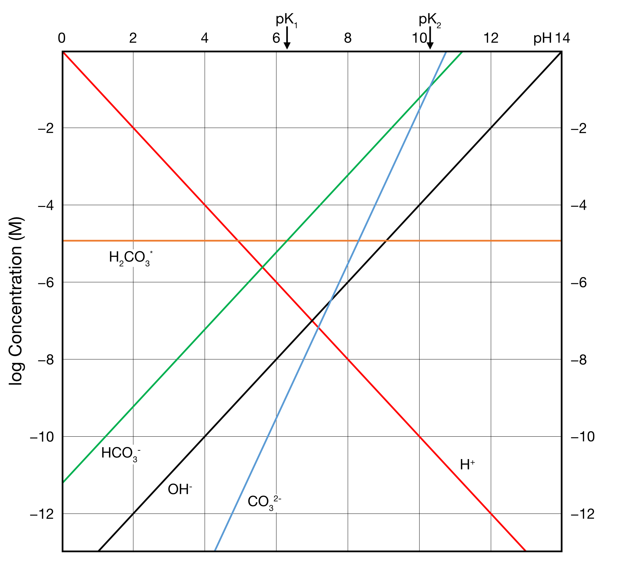
Figure 4: Double logarithmic plot of the equilibrium composition of seawater in our model. Adapted from Stumm and Morgan (1996).

Exercise 3

This is the cool part. Here we are going to calculate a new pH given an increased atmospheric CO₂ concentration. Given that we calculated the concentrations of all the other species according to the initial distribution in Exercise 1, we now hold them all constant, while increasing CO₂ and calculating H⁺ (and therefore pH). This is not simple, because H⁺ concentration is tightly bound up with the concentrations of all other species, and so we cannot simply work backwards from any one equation alone. However, there is a quadratic Equation (29) that we can solve for H⁺ , using a fixed \(C_{T}\), rearranged to Equation (30).

\[\begin{align*} {\left[\color{#FF0000}{H^+}\right]^2C}_T &=\color{#ED7D31}{H_2{CO}_3^\ast}\left(\left[\color{#FF0000}{H^+}\right]^2+K_1\left[\color{#FF0000}{H^+}\right]+K_1K_2\right) \tag{29} \\ \left[\color{#FF0000}{H^+}\right] &=\sqrt[2]{\frac{\color{#ED7D31}{H_2{CO}_3^\ast}}{C_T}\left(\left[\color{#FF0000}{H^+}\right]^2+K_1\left[\color{#FF0000}{H^+}\right]+K_1K_2\right)} \tag{30} \\ \end{align*}\]

Solving this quadratic would be fiendishly difficult. Instead, we will use trial and error, otherwise known as our iterative solution. We will do this to find a value for H⁺ that is the same on both sides of the equation.

\[\begin{equation} \left[\color{#FF0000}{{H^+}_{i}}\right] = \sqrt[2]{\frac{\color{#ED7D31}{H_2{CO}_3^\ast}}{C_T}}\left(\left[\color{#FF0000}{{H^+}_{i-1}}\right]^2+K_1\left[\color{#FF0000}{{H^+}_{i-1}}\right]+K_1K_2\right) \tag{31} \end{equation}\]

Go to the third tab and copy over all of the equations from Exercise 1. The grey boxes are the values that we will hold constant, and the first guess for H⁺, based on the H⁺ in Exercise 1. You can alter the CO₂ concentration using the CO₂ multiplier cell and your rapidly developing Excel and R skills. If you want to double CO₂ concentration, type 2 into the multiplier cell. If you want to keep it at present levels, type 1. Repeat the calculation of Equation (30) over successive iterations, using the answer from the previous iteration as your guess for the next iteration. Eventually, the difference between your guesses will become very small and you can settle on a constant pH. (This is roughly how equilibrium-solving computer programs solve complex biogeochemical interactions, often with many more interacting variables than this.) Don’t forget that your successive iterations, are not time steps, like we had in previous weeks. Rather, they are just guesses at the right number that only exist in the model. Your final answer is the only one that has a real scientific meaning. If you want to determine the pH over a range of CO₂ concentrations, you will need to repeat the calculation over ~10 rows, and save your results each time.

Big questions: if you increase CO₂, does the pH rise or fall? Does CaCO₃ precipitation become more or less favourable if CO₂ increases?

Exercise 4

Last exercise! In this exercise, we will extract someone else’s data from their plot and make our own plot.

Go to the IPCC website and read about CO₂ predictions and CaCO₃ precipitation. Save their Figure 10.24 as an image file or download it here.

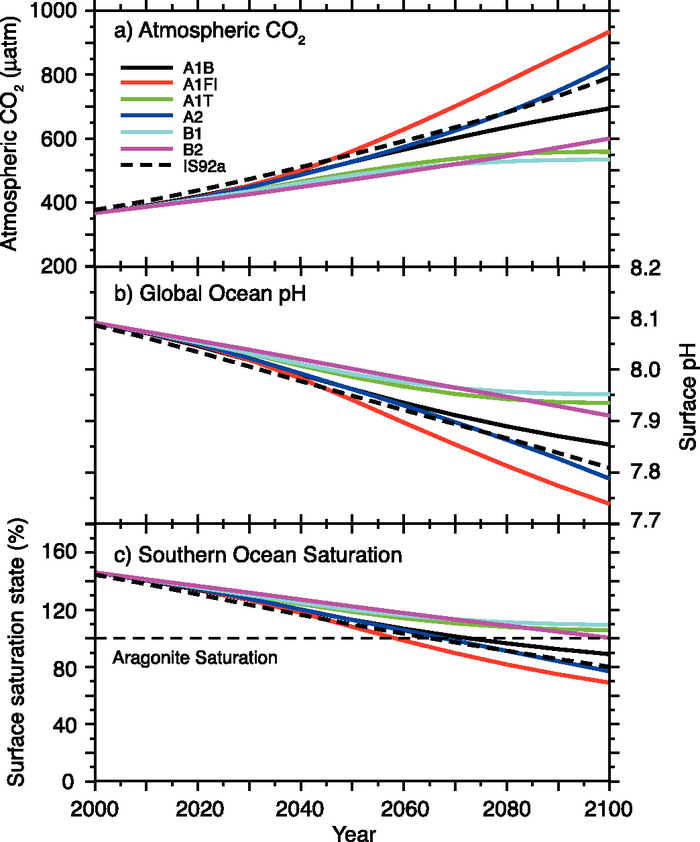
Figure 5: Changes in global average surface pH and saturation state with respect to aragonite in the Southern Ocean under various SRES scenarios.

You can get the data from this figure by uploading it into the Plot Digitizer web app.

(If you want to download the program to work offline, go to the Plot Digitizer website and download the program.)

When this image is loaded into the digitizer, drag the little blue circles for X1 and X2 to the limits of the x axis (2000 and 2100). Type the x axis limits to the panel on the right. You can then set the x axis to be a date axis, using the dropdown. Drag the little red circles the limits of one of the y axes. Enter the limits of the y axes, as seen in the figure, into the panel on the right. Pick one of the coloured lines and add points by clicking along the line. Your points should appear on the left panel. It will be easiest if you make a point every 10 years. If your x-axis points line up nicely enough, you can re-plot the data. You can export the data using one of the grey buttons in the top left, for example, copying it into Excel, or downloading it as a csv. Digitise all three of the datasets, CO₂, pH and omega, and use the same IPCC model for each.

Compare these results with your own results. You will notice the IPCC data graphed over time. Our model depicts an increasing CO₂ environment via the multiplier. The fundamental relationships between these variables is similar - an increasing CO₂ world leads to increased ocean acidification and decreased pH.

Remember back to Module 1 where we modelled salinity values from flow. Let’s do something similar here to make a statistical relationship between year and CO₂ from the IPCC data of CO₂/Year (i.e. use a scatterplot and add a trendline). Use the equation to generate modelled year values for our Exercise 3 model (i.e., we will find out the years that correpsond with our modelled CO2 levels). Finally, you need to predict pH and Omega values from CO₂ values.

You will need to convert atm to µatm and multiply Omega by 100 to create a percentage!

Exercise 5 (Optional)

In this exercise, we will explore the use of AI to assist with the jobs of digitising the data and making comparison plots. To do this we will repeat Exercise 4 using help from an AI chatbot in any way that works well for you. Options can include:

• ChatGPT, or another large language model in a web browser
• the Microsoft Copilot app
• Copilot in Teams / chat
• Copilot in Visual Studio Code

Repeat Exercise 4 with the following steps:

• load the image into the chatbot
• tell the chatbot to digitise one of the lines of the data
• tell the chatbot to digitise all three of the datasets

You can then export that data from the chatbot to Excel and process it there.

We can get further assistance by proceeding within the chatbot and tell it to create the statistical relationship between CO₂ and Year - so we can find the years that align with our model CO2 concentration levels. You can tell the chatbot to create plots of CO₂ on the x axis and Year on the y axis. It will try to create the plot using python.

Finally, you can add your data from the main exercise of this module to the data from the IPCC image. Load your data into the chatbot and tell it to plot both data-sets on the same figure.

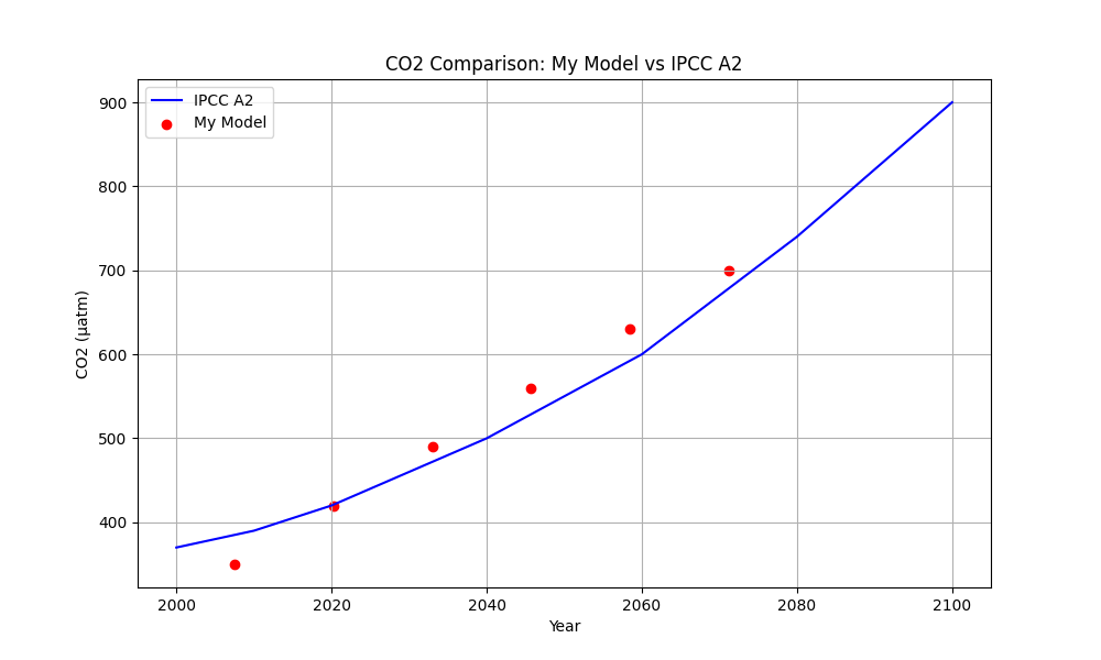
Figure 6: Example AI generated plot.

Writing good prompts is key to either getting AI to do good work for us, or having a frustrating argument with your computer. You need to set the context and guide the chatbot through the steps, at the right pace.

Try writing one complete prompt that tells the chatbot how to do all of the steps.

• Paragraph 1 – Context and Task: Describe what the figure or dataset contains and clearly state what you need to have extracted or analysed.
• Paragraph 2 – Assumptions: Explain how to handle missing or unclear information so the task can still be completed.
• Paragraph 3 – Required Outputs: List your required deliverables in detail, including file formats, content, and any analyses or visualizations.
• Paragraph 4 – Optional Comparison Step: Describe what to do if additional data is provided, including how to compare or combine it with the extracted results.
• Paragraph 5 – Output Format and Code: Explain how the results should be presented and specify any requirements for providing code, or making the work reproducible.

For example (you would need to update the bold items to be specific in your prompt):

I will provide an IPCC figure with three panels: var1 (units), var2, and var3 (units) for multiple SRES scenarios from 2000 to 2XXX. Visually extract data points from a scenario of my choice every 10 years (2000, 20XX, …, 2XXX). If axis ticks cannot be read, use default ranges: CO2 XX–XX, pH X.X to X.X (inverted), Omega XX–160. Return: Three CSVs for the chosen scenario (var1.csv, var2.csv, var3.csv) and a combined CSV (ipcc_digitized_combined.csv with columns Variable ∈ {var1,var2,var3}, Scenario=, Year, Value). Plots for var1, var2, and var3 showing the reconstruction for the chosen scenario. Make a linear regression for Year ~ var1 using the chosen scenario, reporting slope, intercept, and R², plus a scatter-with-fit plot. If I provide a CSV with columns CO2_uatm, pH, and Aragonite_pct, use the regression equation to predict Year from CO2_uatm, and compare the predictions with the extracted scenario data (variable and year) by creating comparison plots (where data from the CSV is plotted as circle markers and the digitised SRES data is as lines; use “My Model” and “IPCC ” as legend entries respectively). Also provide the data as CSVs. Display all results inline and then provide Python code (pandas, numpy, matplotlib) that reproduces the CSVs and plots from the returned tables.

NOTE: You will most likely find that there are some aspects that don’t look right! e.g. the digitised data may not actually look accurate when you comapre to what you manually digitised, or other issues will pop up! In fact, even if you do the same prompt sequence twice you’ll likely get different results 😱 . This is why we ask to receive the python script, as in most circumstances you would then use this as a starting point for your own work, and you would carefully refine the script and data to ensure it was accurate.

Please see the instructions in the Supporting Material on learning to plot with python, and learning to plot with python and AI.

Submission

Submit properly formatted graphs and tables of the following sections of the lab:

1. Double log plot.
2. Your Exercise 3 CO₂ plot comparing your modelled CO₂ and Omega. Attempt to incorporate the IPCC data into this plot.
3. In 3 plots, compare your modelled data with the IPCC data over time (CO₂, pH, and Omega).
4. In 150 words or less, which factors cause the differences between your results and those of the IPCC models.

These are to be uploaded as per the formatting specified in the Style Guide. Marks will be deducted for incorrect formatting.

References

Stumm, Werner, and JJ Morgan. 1996. “Chemical Equilibria and Rates in Natural Waters.” Aquatic Chemistry 1022.