14 Sediment Biogeochemistry

14.1 Contributors

Daniel Paraska, Matthew R. Hipsey

14.2 Overview

This module is a sediment reactive transport model, based on a 1D approximation of the sediment solid and pore-water profiles. Each active sediment zone (or column) is discretized into a user defineable number of layers that start at thicknesses of around 1 mm at the sediment-water interface and increase exponentially down to a pre-defined sediment depth. The model resolves in each layer both physical processes (e.g. pore-water diffusion or bioturbation) and chemical processes (e.g. redox transformations).

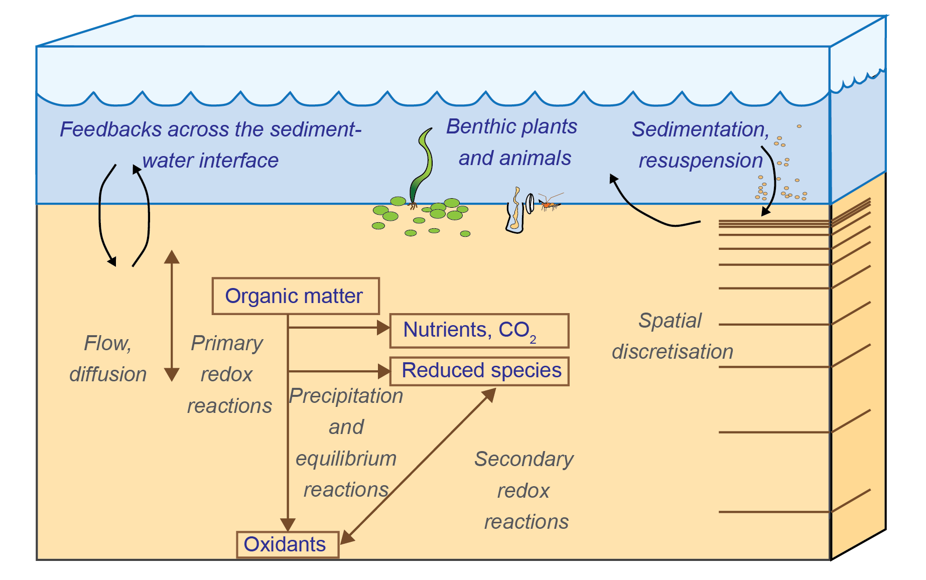
Schematic of the main physical and chemical processes that cause chemical concentration and flux change in the sediment and across the sediment-water interface, and therefore are included in most sediment diagenesis models.

Figure 14.1: Schematic of the main physical and chemical processes that cause chemical concentration and flux change in the sediment and across the sediment-water interface, and therefore are included in most sediment diagenesis models.

Under some conditions, the sediment stores can release nutrients to the water column, while under other conditions, the sediment can remove nutrients, through burial over the long-term, and through processes such as denitrification in the surface layers. The fine balance that controls the conditions under which the sediment will store, release or remove nutrients is largely governed by the aerobic state of the sediment pore water, and the amount of reactive organic matter fuelling the reactions. The depth-resolved sediment model accounts for mixing from the hydrodynamic model into the upper sediment layers, and then calculates whether organic matter is consumed aerobically, through denitrification or, deeper down, through sulfate reduction or even methanogenesis.

Sediment early-diagenesis models are complex environmental reactive transport simulation tools. The meta-analysis by Paraska et al. (2014) discussed the history of their evolution to these complex configurations, in which the original models of Boudreau (1996), Van Cappellen and Wang (1996) and Soetaert et al. (1996) were taken up and applied in many contexts by new modellers, who added new features and extended their capabilities, or discarded old features as required. The meta-analysis also identified the major challenges associated with developing new sediment diagenesis models. Here, the AED modelling package for sediment biogeochemistry is presented, CANDI-AED, which is an extension of the Approach 1 models, but reengineered and augmented with new model approaches and capabilities as a way to address some of these challenges.

Paraska et al. (2015) outlined the significance and uncertainty associated with different parameterisation approaches of organic matter dynamics. In these cases, simulations were run to test the significance of different theoretical approaches and model structural assumptions, using an idealised model setup with only primary oxidation reactions and no physical processes or spatial resolution. The true impact of these different model approaches within a spatially-resolved model, accounting for all of the advection, diffusion and secondary reaction processes, however, is yet to be determined and it is unclear whether some formulations may suit some application contexts better than others. Therefore there is a need for a fully flexible model structure that can include these different organic matter breakdown parameterisations and allow users to assess critically the alternative approaches. In addition, other aspects related to secondary redox reactions, mineral reactions, precipitation and adsorption should similarly be subject to comparative assessments.

The model included in AED aimed to address challenges of building a generic and full-featured, open-source model code with the flexibility to do the following:

set different kinetic rate equation approaches
set different organic matter pools and breakdown processes
use standard inhibition or thermodynamic limits on primary oxidation
optionally use manganese, iron and iron sulphide reactions
simulate adsorbed metals and nutrients
simulate calcium, iron and manganese carbonates
connect the boundary to either another model, a programmed file or a fixed concentration

Therefore the numerical model presented in this module has many optional features and alternative parameterisations for key processes, without mandating their inclusion in the calculations or enforcing a fixed model structure.

The sediment model CANDI-AED presented here is implemented as an optionally configurable module in the AED model library. Through the model coupling approach it may be applied with any of the hydrodynamic models linked to AED (e.g. GLM, Tuflow), or alternatively, options to run in isolation are also possible. This chapter provides a scientific description of the model and describes attributes of the model associated with its practical implementation and operation. A case-study of the model framework is also demonstrated.

The major output of CANDI-AED includes concentration depth profiles and fluxes across the sediment-water interface (figure 14.2).

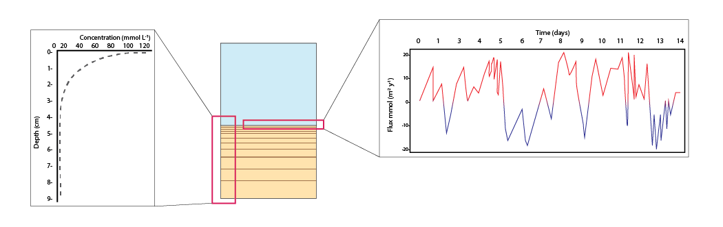
Figure 14.2: Examples of the final outputs after running CANDI-AED: concentration-depth profiles and flux-time plots.

14.3 Model Description

14.3.1 General description

The heart of this model is the reaction, diffusion, advection model of Berner (1980), which was implemented as the Carbon and Nutrient Diagenesis model of Boudreau (1996), later further developed as the C.CANDI code (Luff et al. 2000). The CANDI-AED implementation, however, has evolved from the original code, and includes extensions related to the treatment of organic matter, the simulation of the geochemical conditions known to influence the diagenetic equations, extensions for nutrients and trace metals, and dynamics at the sediment-water interface. However, the core organic matter breakdown equations (and their numerical solution) remains similar as the original descriptions presented in Boudreau (1996), and to other similar sediment models. An overview of the model is shown in Figure 14.3.

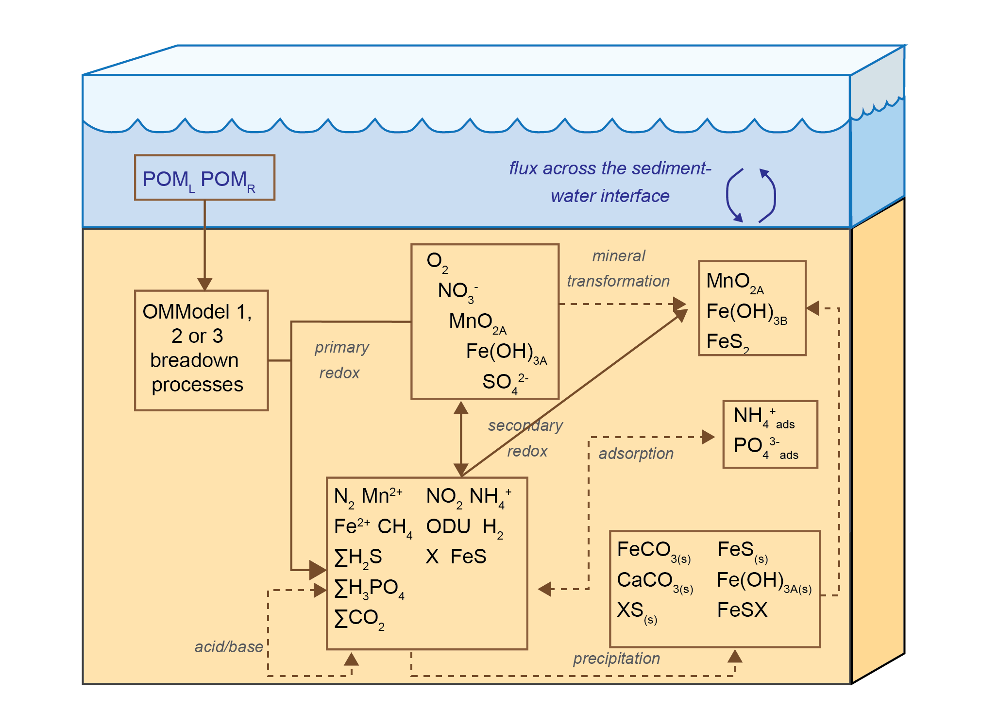
Overview of the chemical processes in CANDI-AED: organic matter transformation and oxidation, and reduction/oxidation, crystallisation, adsorption and precipitation reactions of inorganic by-products. Most of the processes are triggered by the input of POM at the sediment-water interface.

Figure 14.3: Overview of the chemical processes in CANDI-AED: organic matter transformation and oxidation, and reduction/oxidation, crystallisation, adsorption and precipitation reactions of inorganic by-products. Most of the processes are triggered by the input of POM at the sediment-water interface.

The model is based on the advection-dispersion reaction equation for the concentration of dissolved and particulate substances. For dissolved substances $C_d$, the balance equation is defined as:

\[\begin{equation} \frac{\phi \delta C_d}{\delta t} = \overbrace{ D_{B}\frac{\delta^{2} C_d}{\delta x^{2}} + \phi D_{S}\frac{\delta^{2} C_d}{\delta x^{2}} }^\text{biodiffusion and molecular diffusion} - \underbrace{u \frac{\delta C_d}{\delta x}}_\text{advection (flow)} + \overbrace{\alpha(C_{d_0}-C_d)}^\text{irrigation} + \underbrace{\phi \sum R_d}_\text{reactions} + \color{brown}{S} \tag{14.1} \end{equation}\]

where the left hand side (LHS) is the “unsteady” term ($C_d$ change in time), the first term on the right hand side (RHS) is the dispersion/mixing term, the second term on the RHS is the advection/movement term, and $R_d$ denotes a generic reaction term. An optional $S$ term is included to represent sources from other modules (e.g., seagrass root injection of $O_2$).

For particulate (solid) substances, $C_s$:

\[\begin{equation} \frac{(1-\phi)\rho \delta C_s}{\delta t} = \overbrace{ D_{B}\frac{\delta^{2}[(1-\phi)\rho C_s] }{\delta x^{2}} }^\text{biodiffusion} - \underbrace{\omega \frac{\delta [(1-\phi)\rho C_s]}{\delta x}}_\text{advection (sedimentation)} + \overbrace{(1-\phi) \sum R_s}^\text{reactions} + \color{brown}{S} \tag{14.2} \end{equation}\]

where $(1-\phi)$ denotes the solid fraction of the sediment, and $R_s$ is a generic reaction term.

The above equations are solved numerically for the simulated set of constituents. The user can define the variables that are included in the $\mathbf{SDG}$ module, such that $C_d$ and $C_s$, are the set of dissolved and particulate variables selected for simulation, respectively. Eight of the variables (compulsory variables) must be requested by the user in the variable setup file, or the model will not run (see the variables summary below). Three other compulsory variables are always simulated and the user does not need to request them. The other variables can be requested if the user desires them. A number of options are available for resolving the physical processes, including the rate of diffusion, advection, irrigation and the boundary condition options.

In addition to physical processes, the CANDI-AED model considers two types of chemical reactions - the slow, kinetically controlled reactions, and the fast thermodynamically based equilibrium reactions. The latter are simulated in the sediment through appropriate configuration of the geochemistry reactions; the configuration of the equilibrium model will apply to both the water and each of the sediment layers. The kinetically controlled reactions are mostly microbially-mediated and include the reactions for organic matter breakdown and eventual oxidation, the re-oxidation of various by-products and the dynamics of the metal sulfides. These reactions can be complex and are outlined in further detail in the next sections.

14.3.2 Process Descriptions

14.3.2.1 Sediment model domain

The sediment model is discretised into a user-definable number of depth layers (maxnpts) down to a pre-defined sediment depth(xl). The grid of layers is set to have either even spacing (job = 1) or to be exponentially increasing (job = 0), where the layers sizes have a thickness of a few mm at the sediment-water interface and which increase exponentially down into the sediment (figure 14.4). When the spacing increases exponentially, the first two layers are hard-coded to be a miniumum of 0.25 cm, in order to avoid numerical instability from sharp concentration differences over distances that are too small.

This fixed depth of sediment has a concentration of all variables at all depth layers, and boundary conditions at the upper and lower ends of the domain.

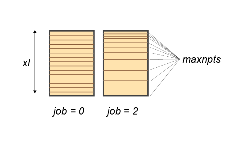
Initialisation of the depth layers. The number of layers is set by `maxnpts` and the depth of the simulation by `xl`. The setup can have even spacing (left) using parameter `job` = 1 or increasing spacing (right) `job` = 2.

Figure 14.4: Initialisation of the depth layers. The number of layers is set by maxnpts and the depth of the simulation by xl. The setup can have even spacing (left) using parameter job = 1 or increasing spacing (right) job = 2.

14.3.2.2 Physical Transport

Solids

CANDI-AED adopts the approach of Boudreau (1996) to advection and dispersion, which is similar to most other diagenesis models. Advection of the solid sediment matrix is occurs at the rate of sediment deposition ($\omega_{00}$ in cm y^-1). The sediment does not move, however, since the height of the modelling domain is fixed, as more sediment accumulates at the surface, a sediment particle moves downwards. An alternative way to view this is that the modelling domain moves upwards.

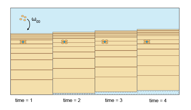
Upon sedimentation, the frame of reference shifts upwards. The bottom area is effectively lost from the modelling domain over time. Particles and porewater are advected downward relative to the modelling domain.

Figure 14.5: Upon sedimentation, the frame of reference shifts upwards. The bottom area is effectively lost from the modelling domain over time. Particles and porewater are advected downward relative to the modelling domain.

Porewater

For the porewater components, diffusion coefficients are used that are based on free-solution molecular diffusion constants corrected for sediment tortuosity, $θ$. Porewater moves downwards at the same rate as the solids ($\omega_{00}$). A further porewater advection term (poreflux) is available, which could represent, for example, pressure on the sediment from a groundwater source. If poreflux is positive, then porewater moves upwards, relative to particles. Conversely, if poreflux is negative, then the porewater moves downwards relative to the particles. In most simulations, poreflux is zero and advection is the transport process. A dynamic poreflux can be assigned using the column headings w00h00 in swibc.dat or pf in deepbc.dat (see setup section below).

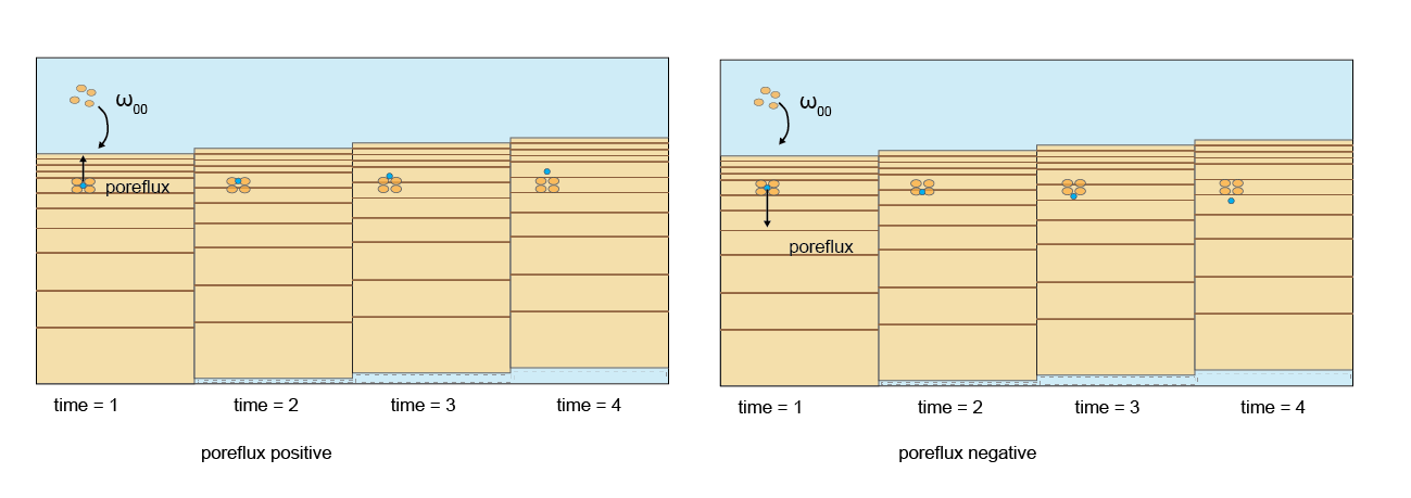
Figure 14.6: Porewater is advected at the same rate as burial. If poreflux is non-zero, an additional rate of advection is applied to porewater. The direction is upwards when poreflux is positive, downwards when poreflux is negative.

Diffusion of solutes is calculated using a diffusivity constant. One default value, which is temperature-dependent, is used for most dissolved variables (table 14.1). This value is based on the diffusivity of chloride. Twelve other variables have their own values, which are also temperature-dependent. Some also use the function a, which can also include salinity and pressure (table 14.1).

Table 14.1: Temperature-dependent calculations for diffusivity constants. All state variables in CANDI-AED use the default value, unless specified in this table. The function a is a further correction for salinity and pressure.
Variable	Diffusivity (cm y^-1)
Default	(9.60 + 0.438×Temperature)×10^-6
O₂	7.4×10^-8(a/25.6^0.6)
CO₂	7.4×10^-8(a/34.0^0.6)
DIC	(5.06 + 0.275×Temperature)×10^-6
NH₄⁺	0.5 × (9.5 + 0.413×Temperature)×10^-6 +
	0.5 × (7.4×10^-8(a/25.8^0.6))
HS^-	0.5 × (10.4 + 0.273×Temperature)×10^-6) +
	0.5 × (7.4×10^-8(a/32.9^0.6))
NO₃^-	(9.50 + 0.388×Temperature)×10^-6
PO₄^3-	0.14 × ((2.62 + 0.143×Temperature)×10^-6) +
	0.85 × ( (3.26 + 0.177×Temperature)×10^-6) +
	0.01 × ( (4.02 + 0.223×Temperature)×10^-6)
Fe²⁺	(3.31 + 0.150×Temperature)×10^-6
Mn²⁺	(3.18 + 0.155×Temperature)×10^-6
SO₄^2-	(4.88 + 0.232×Temperature)×10^-6
CH₄	7.4×10^-8(a/37.7^0.6)

Porosity

Porosity ($\phi$) is defined as the amount of water per total volume of space, as a real number between 0 and 1. A value for porosity is set at each depth layer during initialisation (see initialisation section below) and remains constant throughout the simulation (Figure 14.7). The porosity array is used in the model to calculate other variables, such as

advection
poreflux
porewater volume
solid volume
diffusive velocity
solid fraction

Porosity is also used in the model to calculate $ps$, $psp$ and $pps$, which are used to convert between solid and dissolved state variables, using these conversions:

\[\begin{eqnarray} ps = 1 - \phi \\ \tag{14.3} \\ psp = \frac {ps} {\phi} \\ \tag{14.4} \\ pps = \frac {\phi} {ps} \tag{14.5} \end{eqnarray}\]

Porosity is configured by setting three parameters: the porosity at the sediment-water interface (p0), the porosity at the depth where compaction causes constant porosity with depth (p00), and the attenuation coefficient on the exponential curve (bp) (equation (14.6)). These parameters are set separately for each zone in aed_candi_params.csv. Porosity is the amount of water per total volume of space, as a real number between 0 and 1.

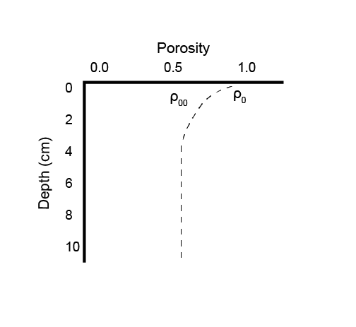
\[\begin{eqnarray} \phi = (\rho _0 - \rho _{00}) \times e^{-bp \times depth} + \rho _{00} \tag{14.6} \end{eqnarray}\]

Figure 14.7: Example depth profile of porosity.

Porosity and bioirrigation profiles are output in the file Depths.sed, along with the depths (in cm), and so the user can examine the shapes of the profiles with depth.

14.3.2.3 Primary Redox Reactions

The key chemical process that causes ongoing change in the sediment is the breakdown of organic matter. Organic matter supplies fuel, above all, reduced carbon, to microorganisms living in the sediment.

Organic matter pools and reactivity

Organic matter ($OM$) degradation pathways can include labile and refractory components, and the breakdown pathways simulated are summarized conceptually in Figure 14.8. Reactions included in the kinetic component include the hydrolysis of the complex (e.g., high molecular weight) $OM$ pools ($POM_{VR}$, $POM_R$, $DOM_R$, $POM_L$) and transformation of low molecular weight (LMW) $DOM_L$ by oxidants ($O_2$, $NO_3^-$, $MnO_2$, $Fe(III)$ and $SO_4^{2-}$ - the so-called ‘terminal metabolism’ pathway), and the release of resulting nutrients ($NH_4^+$, $PO_4^{3-}$) and reduced by-products ($Mn^{2+}$, $Fe^{2+}$, $N_2$, $H_2S$, $CH_4$) and $CO_2$. Oxidants, nutrients and by-products are all capable of interacting, for example, through re-oxidation of reduced species (outlined in the secondary redox section below).

The user can decide how complex or simple the organic matter breakdown pathway should be, with three options of varying complexity for parameterising the pathways included (Figure 14.8). The first option (OMModel = 1) is a common multi-G model in which the $POM$ phases are decomposed straight to $CO_2$ and other breakdown products. Here $POM$ is a variable that is not precisely defined, and its components (such as C, N and P) are assigned by parameters based on a user-defined stoichiometry. OMModel 1 has a switch VCW (logical) that replaces the kinetic rate constants for $POM$ with a depth-dependent breakdown rate, as used by Van Cappellen and Wang (1996).

The second option (OMModel = 2) is another ‘2G’ model with both particulate and dissolved organic matter ($POM$ and $DOM$) phases included and parameterisation hydrolysis of $POM$ to $DOM$, and then $DOM$ to $CO_2$ and other breakdown products. The $POM$ and $DOM$ phases consist of three variables each, which trace the reaction and transport of carbon, nitrogen and phosphorus, thereby allowing for variable stoichiometry of organic matter to occur temporally and spatially.

The third option (OMModel = 3) has many $POM$ phases, which are all hydrolysed to $DOM$, which then undergoes fermentation and terminal metabolism. This allows the carbon, nitrogen and phosphorus to be calculated precisely before and after a model run, and allows the free energies of the reaction of each phase to be included. This third option is the most detailed and mechanistic, and allows for expansion of more detailed reaction mechanisms to be included, but is recommended only for experienced users.

CANDI-AED also contains options for very unreactive organic matter parameter. The model can decrease the reactivity of the particulate refractory phase towards zero as the concentration approaches a minimum. For example, for $POC_R$, the parameter pocu sets the minimum concentration and KOMPres_C sets the sensitivity of the decrease, as in equation (14.7) below. The equivalent parameters for N an P are ponu and popu, and KOMPres_N and KOMPres_P.

\[\begin{eqnarray} komlim = \frac {PON_R - ponu} {PON_R - ponu + KOMPres_N} \\ \\ R_{PONR} = (ponr2donr) (komlim) \tag{14.7} \end{eqnarray}\]

(The equation above is a simplified version, where the full equation had checks to prevent the rate going below zero, plus the respiration processes of $MPB$.)

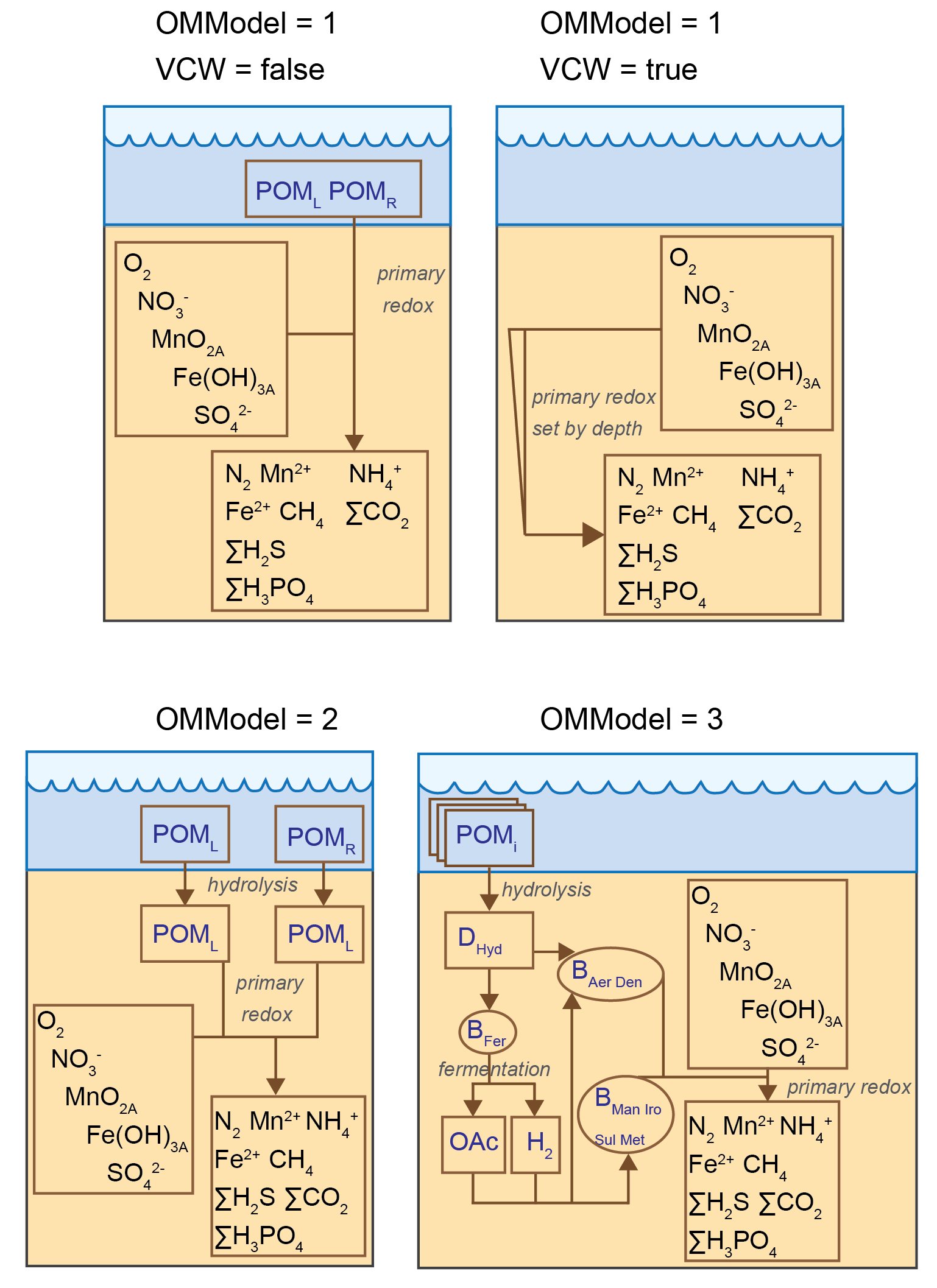
Three options for different levels of complexity in organic matter breakdown, by setting the `OMModel` switch. Top left – Model in which $POM$ breaks down directly to $CO_2$ and other waste products. Top right - Model with the breakdown rate set by depth. Bottom left – Model in which POM is first hydrolysed to $DOM$ and then oxidised to $CO_2$. Bottom right – Model in which $POM$ is hydrolysed to $DOM$, which can then be fermented and oxidised.

Figure 14.8: Three options for different levels of complexity in organic matter breakdown, by setting the OMModel switch. Top left – Model in which $POM$ breaks down directly to $CO_2$ and other waste products. Top right - Model with the breakdown rate set by depth. Bottom left – Model in which POM is first hydrolysed to $DOM$ and then oxidised to $CO_2$. Bottom right – Model in which $POM$ is hydrolysed to $DOM$, which can then be fermented and oxidised.

Table 14.2: Organic matter breakdown processes. The index i in *∑ R_Oxi* refers to the sequence of *TEA* in table 14.3">. For `OMModel` 2, $POM$ and $DOM$ are each three state variables of $POC$, $PON$ and $POP$, and $DOC$, $DON$ and $DOP$.
Description	Reaction	Rate equation
OMModel 1
POM_Lab oxidation	POM_Lab $\rightarrow$ CO₂ etc.	poml2dic ∑R_Oxi
POM_Ref oxidation	POM_Ref $\rightarrow$ CO₂ etc.	pomr2dic ∑R_Oxi
POM_Ref oxidation	POM_Ref $\rightarrow$ CO₂ etc.	pomspecial2dic ∑R_Oxi
OMModel2
POMLab hydrolysis	POM_Lab $\rightarrow$ DOM_Lab	pocl2docl (POC_L)
POMRef hydrolysis	POMRef $\rightarrow$ DOM_Ref	pocr2docr (POC_R)
DOMLab oxidation	DOMLab $\rightarrow$ CO₂ etc.	docl2dic ∑R_Oxi
DOMRef oxidation	DOMRef $\rightarrow$ CO₂ etc.	docr2dic ∑R_Oxi
OMModel 3
POMi hydrolysis	POMi $\rightarrow$ D_Hyd	k~POM i~ (POM_i)F_BHyd
DHyd fermentation	DHyd $\rightarrow$ OAc + H₂	k_growthB_FerF_T _FerF_DHyd
DHyd oxidation	DHyd $\rightarrow$ CO₂ etc.	k_growthB_Aer,DenF_T _j F_DHyd
OAc, H2 oxidation	OAc, H2 $\rightarrow$ CO₂ etc.	k_growthB_jF_T _j F_TEA _jF_OAc,H2 F_In _j
OMModel 4
POM oxidation	POM $\rightarrow$ CO₂ etc.	R₀ e^(-$\beta$ ^$\times$ ^depth)

C:N:P partitioning

The C:N:P stoichiometry is set differently for each OMModel.

Using OMModel = 1, the ratios are set separately for the labile and refractory phases, using the x, y and z ratios outlined in table 14.3. For example, xlab is the carbon fraction of $POM_L$, which is usually set to around 106, while zlab is the $POM_L$ phosphorus fraction, which is usually set to around 1. These ratios are fixed throughout the simulation. The x, y and z coefficients are used to set the proportions of the other species in the redox equation (such as oxidants and reduction products), the acid-base products (such as $HCO_3^-$ and $CO_2$) and the amounts of free $NH_4^+$ and $PO_4^{3-}$ released from organic matter degradation oxidation.

The x, y and z ratios in table 14.3 are written in the standard form of the equations in the sediment model literature. The carbon in the organic matter is assumed to be carbon (0) and each carbon atom requires four electrons from the oxidant to form the carbon (IV) in $CO_2$, and therefore x carbons require 4x electrons. In practice, the model code performs reactions per carbon, and so all of these coefficients are divided by x, for all reactants and products. This is done in order to make the reactions OMModel 1 equivalent to OMModel 2.

Using OMModel = 2, the C:N:P ratio is set by the concentrations of separate organic species, such as $POC_L$, $PON_L$ and $POP_L$, as opposed to the $POM$ phases of OMModel 1. The ratio is fixed by the boundary and initial conditions, however, if the boundary is dynamic, then the ratio can change through the course of the simulation. Only $DOC_L$ participates in the redox reactions, and so the equivalent of CH₂O in table 14.3 is $DOC_L$. The release of organic N as free $NH_4^+^$ is calculated $PON_L$ oxidation at ponl2dic and the release of organic P as free $PO_4^{3-}$ as $POP_L$ at popl2dic.

Using OMModel = 3 is similar to OMModel = 1. The ratios are applied to $POM_1$, $POM_2$ etc. as xPOM1, yPOM2 etc.

The redox sequence

The terminal redox reaction pathways are the six major pathways that are available in most diagenesis models, and are driven by different organic matter pools, depending on the OMModel configuration chosen from the above options. CANDI-AED allows the use of Approach 1 or 2 organic matter oxidation rate equations, as examined in detail in Paraska et al. (2015), and also explained below. The six major pathways are:

Aerobic
Denitrifying
Manganese reduction
Iron reduction
Sulfate reduction
Methanogenesis

The decay of the complex $OM$ types to the LMW $DOM$ required for the heterotrophic bacteria to utilise are all modelled with a simple first-order decay rate. The subsequent reactions for terminal metabolism that describe the breakdown of $OM$ to $CO_2$ and other breakdown products are described in table 14.3.

CANDI-AED uses a more detailed set of reactions for the denitrifying process, which are described in the Nitrogen cycling section below. The chemical equations may be written as in table 14.3 and the reaction rates for each of these are calculated dynamically based on Monod expressions which mediate the reaction rate according to the concentration of potential oxidants higher in the redox sequence, and the concentration of the available oxidant.14.23

Table 14.3: Primary terminal redox reactions. x, y and z are stoichiometric coefficients.
Description	.	Reaction
Denitrousation		$\displaystyle \ (CH_2O)_x(NH_3)_y(PO_4)_z +2x N_2O + (-y + 2z) HCO_3^- \rightarrow 2xN_2 + (x-y+2z)CO_2 + (x-y+2z)H_2O + yNH_4^+ + zHPO_4^{3-}$
Aerobic respiration		$\displaystyle \ (CH_2O)_x(NH_3)_y(PO_4)_z +(x+2y)O_2 + (y + 2z) HCO_3^- \rightarrow + (x+y+2z)CO_2 + (x+y+2z)H_2O + yNH_4^+ + zHPO_4^{3-}$
Denitritation		$\displaystyle \ (CH_2O)_x(NH_3)_y(PO_4)_z +2x NO_3^- + (-y + 2z) HCO_3^- \rightarrow +2x NO_2^- + (x-y+2z)CO_2 + (x-y+2z)H_2O + yNH_4^+ + zHPO_4^{3-}$
Nitrous denitritation		$\displaystyle \ (CH_2O)_x(NH_3)_y(PO_4)_z + 2x NO-2^- + (-2x-y + 2z) HCO_3^- \rightarrow xN_2O + (x-y+2z)CO_2 + (-y+2z)H_2O + yNH_4^+ + zHPO_4^{3-}$
DNRA		$\displaystyle \ (CH_2O)_x(NH_3)_y(PO_4)_z + \frac{2x}{3}NO_2^- + (\frac{-4x}{3} -y +2z )HCO_3^-\rightarrow\\ \\ \frac{2x}{3} NH_4^+ (reduction \ \ product)+ (\frac{-x}{3}-y+2z)CO_2 + (-x-y+2z)H_2O + yNH_4^+ (from \ \ organic \ \ nitrogen) + zHPO_4^{3-}$
Mn oxide reduction		$\displaystyle \ (CH_2O)_x(NH_3)_y(PO_4)_z + 2xMnO_2 + (x + y - 2z) H_2O + (3x + y - 2z)CO_2 \rightarrow 2xMn^{2+} + (4x + y - 2z)HCO_3^- + yNH_4^+ + zHPO_4^{3-}$
Fe oxide reduction		$\displaystyle \ (CH_2O)_x(NH_3)_y(PO_4)_z + 4x FeOOH + (x + y - 2z) H_2O + (7x + y - 2z)CO_2 \rightarrow 4x Fe^{2+} + (8x + y - 2z)HCO_3^- + yNH_4^+ + zHPO_4^{3-}$
Sulfate reduction		$\displaystyle \ (CH_2O)_x(NH_3)_y(PO_4)_z + \frac{x}{2} SO_4^{2-} + (\frac{-x}{2} - y + 2z) HCO_3^- \rightarrow \frac{x}{2}HS^- + (\frac{x}{2} - y + 2z)CO_2 + (\frac{x}{2} - y + 2z)H_2O + yNH_4^+ + zHPO_4^{3-}$
Methanogenesis		$\displaystyle \ (CH_2O)_x(NH_3)_y(PO_4)_z + (- y + 2z) HCO_3^- \rightarrow 0.5 CH_4 + (0.5x - y + 2z)CO_2 + yNH_4^+ + zHPO_4^{3-}$

The kinetic rate constant k_OM gives the maximum oxidation rate, which is different for each reactive organic matter type, but the same for each oxidation pathway.

When using OMModel 3, the kinetic rate constant is the rate of bacterial growth. The rates are calculated as the product of the rate constant, the concentration and a series of limitation and inhibition factors that scale between 0 and 1.

Limitation and inhibition factors

A common feature of all diagenesis models is that the oxidation rate expression $R_{Ox}$ is a product of up to seven terms:

an organic matter reaction rate constant k_OM
the organic matter concentration limitation, $F_{OM}$
a temperature dependence $F_{Tem}$
a microbial biomass factor, $F_{Bio}$
a term limitation factor, $F_{TEA}$
an inhibition term, $F_{IN}$ and
a thermodynamic factor, $F_{T}$
a thermodynamic factor, $F_{an}$

\[\begin{equation} R_{Ox_{i}} = k_{OM}F_{OM}F_{Tem}F_{Bio}F_{TEA{i}}F_{In_{i}}F_{T}F_{an} \\ \tag{14.8} \end{equation}\]

In CANDI-AED, organic matter limitation, $F_{OM}$, is only used with OMModel 3. It takes the general form

\[\begin{equation} F_{OM_{i}} = \frac{OM_{i}} {(OM_{i} + K_{OM})} \\ \tag{14.9} \end{equation}\]

where $OM_i$ is an organic matter species, such as $D_{Hyd}$ or $OAc$ and K_OM is a limiting concentration. This functions like other Monod terms, limiting the reaction rate when the concentration of $OM_{i}$ is low. Using OMModel 1 or 2 (the common and simplest options), $F_{OM}$ is effectively 1 and it is assumed that organic matter concentration never limits the reaction rate.

The temperature factor $F_{Tem}$ is rarely employed in diagenesis models, but in a handful of cases it uses a Q₁₀ relationship between 2 and 4 (see Fossing et al. 2004 for a clear explanation of how temperature affects reaction rates and Eldridge and Morse (2008) or Reed et al. (2011) for a specific examination of the effect of temperature). The current version of the model has switches built in for the temperature dependence factor, $F_{Tem}$, where values of 1 or 2 turn them off and on. However, implementation and testing of the factors has not been carried out for this version of the model.

The TEA factor, $F_{TEA}$, term accounts for the $R_{Ox}$ dependence on the oxidant concentration when the oxidant concentration is low. The $F_{TEA}$ term in Approach 1 is a Monod expression (table 14.4, figure 14.9), which uses Monod half-saturation constants (K_Ox), and which is chosen because it best reflects laboratory data of bacterially-controlled oxidation reactions (Boudreau and Westrich, 1984, Gaillard and Rabouille 1992). In Approach 2, the $F_{TEA}$ is either 0, 1 or the ratio of Ox_i to L_Ox, depending on the oxidant concentration relative to L_Ox, a specified limiting concentration (table 14.4). We use the notation K_Ox and L_Ox to emphasise that a distinction should be made between the Monod half constants in Approach 1 and the limiting concentrations used in Approach 2; the difference in conceptual representation is not always clear in Approach 2 papers that use the notation K_Ox. We recommend that the user set the parameter OMModel to 1, unless they specifically need to emulate an Approach 2 model, such as that by Van Cappellen and Wang (1996).

Table 14.4: Limitation and inhibition equations for the two different approaches (`OMApproach`).
Approach	Limitation factor - FTEA	Inhibition factor - FIn
1	$\displaystyle \ \frac {TEA}{TEA + K_{TEA} }$	$\displaystyle \ \frac {K_{In}} {TEA + K_{In} }$
2	$\displaystyle \ 0, \frac {TEA}{K_{TEA} } or 1$	$\displaystyle \ 1 - \frac {TEA}{K_{In} }$

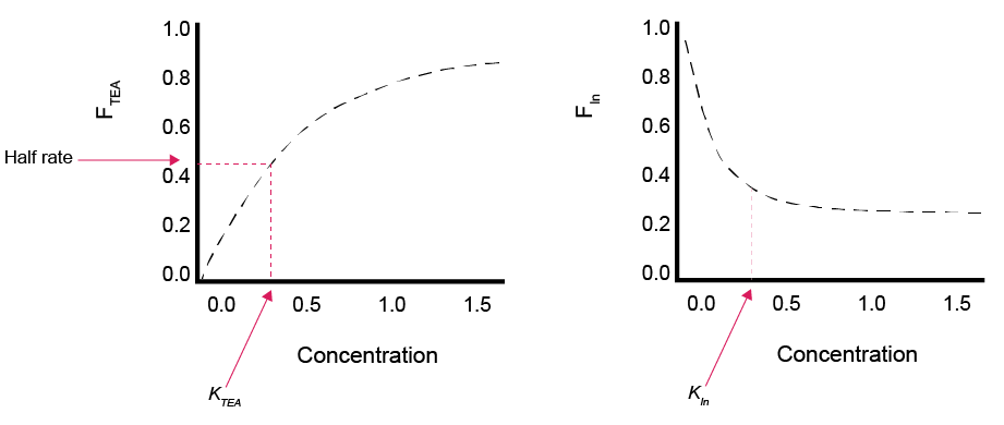
Schematic of examples of how inhibition and limitation scale between 0 and 1 over a range of concentrations. Left: limitation function. Right: inhibtion function.

Figure 14.9: Schematic of examples of how inhibition and limitation scale between 0 and 1 over a range of concentrations. Left: limitation function. Right: inhibtion function.

$F_T$ is the thermodynamic factor. The current version of the model includes $F_T$ only for OMModel 3, for terminal oxidation reactions and fermentation. This factor uses the ratio of products and reactants, as well as the free energy of each reaction pathway ($\Delta G^0$).

The $F_T$ is a factor that scales between 0, which stops the reaction, and 1, which allows the reaction to proceed, in the same way as $F_{TEA}$ and $F_{In}$. The form of the equation proposed by Jin and Bethke is that shown in equation (14.10).The m and χ are stoichiometric coefficients, ΔG_ATP is the energy required to synthesise one mole of ATP, R is the gas constant and T is the temperature. In the case where the $F_T$ < 0 then the factor is set to 0 by convention, otherwise a negative FT would represent the case where microbes carried out a reaction that was unfavourable to their metabolism.

\[\begin{equation} F_T = 1 - e^{\frac {∆G_r + m ∆G_{ATP}} {χR} } \tag{14.10} \end{equation}\]

ΔG_r is the changing free energy in the system, which controls whether the $F_T$ becomes favourable or not as the environment changes, and is calculated according to the simplified version in equation (14.11) (see Jin and Bethke 2005 for a more precise definition):

\[\begin{equation} ∆G_r = ∆G^0 + RT ln ( \frac {[redox \ products]^{molar \ ratios} } { [redox \ reactants]^{molar \ ratios} } ) \\ \tag{14.11} \end{equation}\]

where ΔG₀ is the standard state free energy of a redox reaction, calculated as the sum of the energy of the reduction of a TEA and the oxidation of an organic substrate. These energies are well constrained by laboratory data, though there may be differences between laboratory and field conditions that create some uncertainty in their use (Bethke et al. 2011). Practically, this equation allows for ΔG_r to be very close to ∆G₀ when the reactants are at high concentrations relative to the products. Inversely, when the products are at relatively high concentrations, ΔG_r becomes more positive, making $F_T$ more negative. Equation (14.10) requires the constants m and χ, which are parameters that could be measured empirically, however as yet they have not all been measured for every redox pathway for every substrate, and therefore authors have had to estimate some values when using equation (14.10) (Dale et al. 2008). It also requires ΔG_ATP, which is around 45 kJ (mol substrate)^-1 but has varied published values. Around neutral pH the conditions for fermentation product consumption by iron reducers, sulphate reducers and methanogens are all thermodynamically favourable, but this changes with pH (Bethke et al. 2011). Acidity either promotes or hinders the reaction depending on whether the protons are produced or consumed in the reaction.

$F_{an}$ is a factor that slows down sulfate reduction and methanogenesis. As stated above, the kinetic rate constant k_OM is the same for all redox pathways. The higher-energy pathways are designed to inhibit the lower-energy pathways, but not to occur faster, which is consistent with most other diagenesis models. However, there is an option to slow sulfate reduction and methanogenesis if the user desires. The parameter f_an can be set between 0 and 1 to make the $F_{an}$ factor more or less sensitive. Any value greater than 1 makes the factor ineffective (equation @ref(eq:#factors-4)). The $F_{an}$ factor is calculated as the fraction of $F_{Sul}$ and $F_{Met}$ over the sum of all of the other pathways.

\[\begin{equation} For \ \ R_{O_{2}},\ \ R_{NO_{3}},\ \ R_{MnO_{2}}, \ \ and \ \ R_{FeOH} \ \\ \\ F_{an (factor)} = 1 \\ \\ For \ \ R_{SO_{4}} \ \ and \ \ R_{Met} \ \\ \\ F_{an (factor)} =\left\{ \begin{array}{@{}ll@{}} 1, & f_{an (parameter)} \: \ge \: 1 \\ \frac {F_{SO_{4}} + F_{Met}}{f_{an (parameter)} + F_{O_{2}} + F_{NO_{3}} + F_{MnO_{2}} + F_{FeOH} + F_{SO_{4}} + F_{Met}}, & f_{an (parameter)} \lt 1\\ \end{array}\right. \tag{14.11} \end{equation}\]

Nitrogen cycling

The redox sequence in CANDI-AED is slightly different to the sequence in other diagenesis models: here the nitrogen redox reactions are split into several processes. Most diagenesis models have an overall reaction of $NO_3^-$ oxidising organic matter and producing $N_2$, as shown in figure 14.10. This reaction is less favourable than aerobic oxidation and it is inhibited by $O_2$.

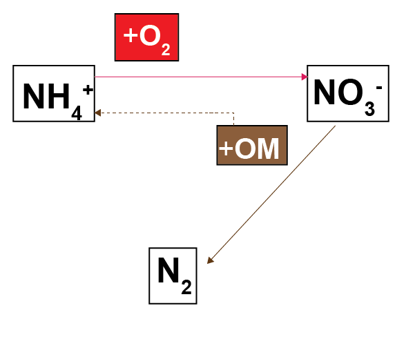
Figure 14.10: Schematic of the basic nitrogen-organic matter redox process from most other diagenesis models.

In CANDI-AED, there are separate nitrogen reactions for oxidising organic matter:

Denitrousation: $N_2O$ reduction to $N_2$
Denitratation: $NO_3^-$ reduction to $NO_2^-$
Denitritation: $NO_2^-$ reduction
Nitrous denitritation: $NO_2^-$ reduction to $N_2O$
DNRA: (Dissimilatory nitrate reduction to ammonia) $NO_2^-$ reduction to $NH_4^+$

These reactions interact as shown in figure 14.11. In CANDI-AED, the denitrousation reaction is configured to be more favourable than aerobic oxidation, based on the free energy data reported in Lam and Kuypers (2011). Therefore $N_2O$ inhibits aerobic respiration and all lower-energy pathways. Denitratation and all other reactions are less favourable than aerobic oxidation. Denitritation is the term used for the oxidation of $NO_2^-$, the products of which are produced through either nitrous denitritation (to $N_2O$) or DNRA (to $NH_4^+$), depending on the abundance of $NO_2^-$.The rate equations are as shown in table 14.5.

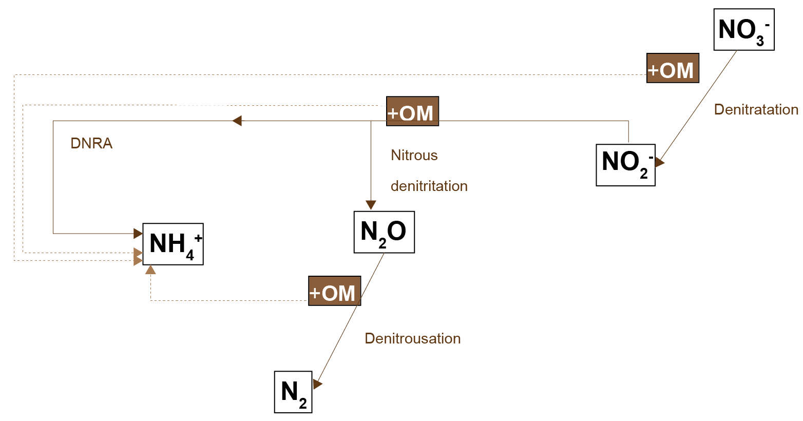
Figure 14.11: Schematic of the nitrogen-organic matter redox processes used in the CANDI-AED model.

Table 14.5: Rate equations for organic matter oxidation by nitrogen.
Process	Rate equation
Denitratation	$\displaystyle \ \ R_{Denitratation} = k_{OM} OM \frac {NO_3^-} {NO_3^- + K_{NO3} } \frac {K_{O2}^1} {O_2 + K_{O2}^1} \frac {K_{N2O}} {N_2O + K_{N2O}}$
Denitritation	$\displaystyle \ \ R_{Denitritation} = k_{OM} OM \frac {K_{O2}^3} {O_2 + K_{O2}^3 } \frac {K_{N2O}} {N_2O + K_{NO2} }$
Nitrous denitritation	$\displaystyle \ \ R_{Nitrous denitritation} = \frac {1} {2} R_{Denitritation} \frac {NO_2^- } {NO_2^- + K_{NO2} }$
DNRA	$\displaystyle \ \ R_{DNRA} = R_{Denitritation} \frac {K_{NO2} } {NO_2^- + K_{NO2} }$
Denitrousation	$\displaystyle \ \ R_{Denitrousation} = k_{OM} OM \frac {K_{N2O} } {K_{N2O}^6 +O_2 }$
Ammonium release	$\displaystyle \ \begin{align} \ R_{Ammonium release} = k_{OM} OM \times \\ (R_{Denitratation} + R_{Denitritation} + R_{Denitrousation}) \times \ \frac {N } {C } \end{align}$

Along with the nitrogen–organic matter redox reactions, there are sets of nitrogen oxidation reactions, where the oxidant is $O_2$ or $NO_2^-$. These are outlined in more detail in the AED inorganic nitrogen chapter.

Calculation of the primary reactions

The chemical reactions in table 14.3 represent the overall process, however, the model code does not contain them in that form. A description of the numerical solution is presented below in the section Numerical solution and a summary of the process as it pertains to primary reactions is given here. The model code contains:

The ‘Reaction’ function: the balance of each reaction rate for each species.

The ‘Rates’ function: the reaction rates, as the product of

the species,
the kinetic constants,
the stoichiometric coefficients and
the factors.

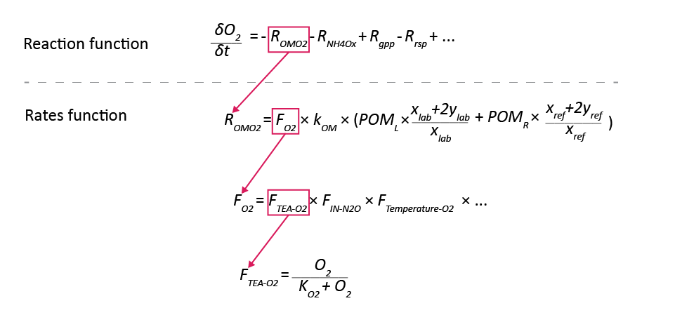
An illustration of one example of how the reaction rates are calculated in the model code. The balance equation is calculated as the gains and losses from the individual rates, and the rates are calculated from constants or other variables.

Figure 14.12: An illustration of one example of how the reaction rates are calculated in the model code. The balance equation is calculated as the gains and losses from the individual rates, and the rates are calculated from constants or other variables.

14.3.2.4 Secondary Redox Reactions

The reactions of chemical species produced by the primary redox reactions (14.6) are referred to as secondary redox reactions, and are usually given bimolecular rate laws, which are first order with respect to the oxidant and reductant (14.6). The rates are controlled by a kinetic constant with units (mmol L)^-1 y^-1.

Table 14.6: Chemical reactions for secondary redox reactions.
Description	Reaction	Rate equation
Simple NH₄⁺ oxidation by O₂	$\displaystyle \ NH_4^++ 2O_2 + 2HCO_3^- \rightarrow NO_3^-+ 2CO_2 + 3H_2O$	$\displaystyle R_{NH4Ox} = k_{NH4Ox}[NH_4^+][O_2]$
Ammonium oxidation	0	$\displaystyle R_{Ammonium \ \ oxidation} = k_{NH4O2}[NH_4^+][O_2]$
NH₄⁺ oxidation by O₂: nitrousation	$\displaystyle \ 2NH_4^+ + 2O_2 + 2HCO_3^- \rightarrow N_2O + 2CO_2 + 5H_2O$	$\displaystyle R_{Nitrousation} = R_{Ammonium \ \ oxidation} \frac{K_{part \ \ ammox}}{K_{part\ \ ammox} + O_2}$
NO₂^- oxidation by O₂: nitratation	$\displaystyle \ NO_2^-+ \frac{1}{2} O_2 \rightarrow NO_3^-$	$\displaystyle R_{NO2O2} = k_{NO2O2}[NO_2^-][O_2]$
NH₄⁺ oxidation by O₂: nitritation	$\displaystyle \ NH_4^++ \frac{3}{2} O_2 + 2HCO_3^- \rightarrow NO_2^-+ 2CO_2 + 3H_2O$	$\displaystyle R_{NH4Ox} = R_{Ammonium \ \ oxidation} \frac{O_2}{K_{part \ \ ammox} + O_2}$
NH₄⁺ oxidation by NO₂^- (Deammonification, anammox)	$\displaystyle \ NH_4^+ + NO_2^- \rightarrow N_2 + 2H_2O$	$\displaystyle R_{NH4NO2} = k_{NH4NO2}[NH_4^+][O_2]$
Mn²⁺ oxidation by O₂	$\displaystyle \ Mn^{2+} + _{Xmk}X+ \frac{1}{2}O_2 + 2HCO_3^- \rightarrow MnO_{2A}-X_{Xmk}+ 2CO_2 + H_2O$	$\displaystyle R_{MnOx} = k_{MnOx}[Mn^{2+}][O_2]$
Fe²⁺ oxidation by O₂	$\displaystyle \ 4Fe^{2+}+ \frac{1}{2}O_2 + 4CO_2 + 2H_2O \rightarrow 4Fe^{3+}+ 4HCO_3^-$	$\displaystyle R_{FeOx} = k_{FeOx}[Fe^{2+}][O_2]$
H₂S oxidation by O₂	$\displaystyle \ H_2S+ 2O_2 + 2HCO_3^- \rightarrow SO_4^{2-}+ 2CO_2 + 2H_2O$	$\displaystyle R_{TSOx} = k_{TSOx}[H_2S][O_2]$
CH₄ oxidation by O₂	$\displaystyle \ CH_4+ O_2 \rightarrow + CO_2 + H_2O$	$\displaystyle R_{CH4Ox} = k_{CH4Ox}[CH_4][O_2]$
FeS oxidation by O₂	$\displaystyle \ FeS-X_{Xfm}+ O_2 \rightarrow SO_4^{2-} + Fe^{2+} + _{Xfm}X$	$\displaystyle R_{FeSOx} = k_{FeSOx}[FeS][O_2]$
FeS₂ oxidation by O₂	$\displaystyle \ FeS_2- X_{Xfm}+ 3.5O_2 + 2HCO_3^- \rightarrow Fe^{2+} + _{Xfm}X +2SO_4^{2-}+ 2CO_2 + H_2O$	$\displaystyle R_{FeS2Ox} = k_{FeS2Ox}[FeS_2][O_2]$
Mn²⁺ oxidation by NO₃^-	$\displaystyle \ 5Mn^{2+} + 2NO_3^- + 8HCO_3^- + _{xmk}X \rightarrow 5MnO_{2A}-_{xmk}X + 8CO_2 + 4H_2O + N_2$	$\displaystyle R_{MnNO3} = k_{MnNO3}[Mn^{2+}][NO_3^-]$
Fe²⁺ oxidation by NO₃^-	$\displaystyle \ 5Fe^{2+} + NO_3^-+ CO_2 + 3H_2O \rightarrow \frac{1}{2}N_2 + Fe^{3+} + 6HCO_3^-$	$\displaystyle R_{FeNO3} = k_{FeNO3}[Fe^{2+}][NO_3^-]$
∑H₂S oxidation by NO₃^-	$\displaystyle \ \frac{5}{2}H_2S + 4NO_3^- + HCO_3^- \rightarrow \frac{5}{2} SO_4^{2-} +2N_2 + CO_2 + 3H_2O$	$\displaystyle R_{TSNO3} = k_{TSNO3}[H_2S][NO_3^-]$
Fe²⁺ oxidation by MnO_2A, _B	$\displaystyle \ 2Fe^{2+} + 21X + (MnO_{2A}-X_{Xmk} + MnO_{2B}-X_{Xmk}) + 2HCO_3^- + 2H_2O \rightarrow 2Fe(OH)_{3A}-X_{xfl} + Mn^{2+} + kX + CO_2$	$\displaystyle R_{FeMn} = k_{FeMn}[Fe^{2+}][MnO_{2A, B}]$
∑H₂S oxidation by MnO_2A, _B	$\displaystyle \ H_2S + 4(MnO_{2A}-X_{Xmk} + MnO_{2A}-X_{Xmk}) + 6CO_2 + 2H_2O \rightarrow SO_4^{2-} + 4Mn^{2+}+ 4 _{Xmk}X + 6HCO_3^-$	$\displaystyle R_{TSMnO2} = k_{TSMnO2}[H_2S][MnO_{2A, B}]$
FeS oxidation by MnO_2A, _B	$\displaystyle \ FeS-X_{Xfm} + 4(MnO_{2A}-X_{Xmk} + MnO_{2B}-X_{Xmk} ) + 8CO_2 + 4H_2O \rightarrow SO_4^{2-} + 4Mn^{2+} + Fe^{2+} + (m + 4Xfm) X + 8HCO_3^-$	$\displaystyle R_{FeSMn} = k_{FeSMn}[FeS][MnO_{2A, B}]$
∑H₂S oxidation by Fe(OH)_3A, _B	$\displaystyle \ H_2S + 8(Fe(OH)_{3A}-X_{Xfl} + Fe(OH)_{3B}-X_{Xfl} ) + 14CO_2 \rightarrow SO_4^{2-} + 9 Fe^{2+} + 8_{XmK} X + 16HCO_3^- + 4H_2O$	$\displaystyle R_{TSFe} = k_{TSFe}[H_2S][Fe(OH)_{3A, B}]$
FeS oxidation by Fe(OH)_3A, _B	$\displaystyle \ FeS-X_{Xfl} + 8(Fe(OH)_{3A}-X_{Xfl} + Fe(OH)_{3A}-X_{Xfl}) + 16CO_2 \rightarrow SO_4^{2-} + 9 Fe^{2+} + (m+8Xfl)X + 16HCO_3^- + 4H_2O$	$\displaystyle R_{FeSFe} = k_{FeSFe}[FeS][Fe(OH)_{3A, B}]$
CH₄ oxidation by SO₄^2-	$\displaystyle \ CH_4 + SO_4^{2-} + CO_2 \rightarrow H_2S + 2HCO_3^-$	$\displaystyle R_{CH4SO4} = k_{CH4SO4}[CH_4][SO_2^{2-}]$
H₂ oxidation by SO₄^2-	$\displaystyle \ 5H_2 +SO_4^{2-} \rightarrow H_2S + 4H_2O$	$\displaystyle R_{HSO} = k_{HSO}[H_2][SO_4^{2-}]$

Calculation of the secondary reactions

As with the primary reactions, the secondary redox reactions are present in the code as the combination of

The ‘Reaction’ function: the sum of the rates of change of each species.

The ‘Rates’ function: the reaction rates, as the product of

the species,
the kinetic constants,
the stoichiometric coefficients and
the factors.

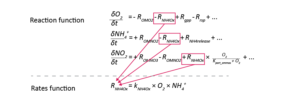
Figure 14.13: An illustration of one example of how the reaction rates are calculated in the model code. The balance equation is calculated as the gains and losses from the individual rates, and the rates are calculated from constants or other variables.

14.3.2.5 Equilibrium Geochemistry

pH

The pH is initialised at a fixed value of around 8, which the user does not control. Setting the parameter rxn_mode to 0 or 4 keeps the pH constant throughout the simulation. Setting rxn_mode to 1, 2 or 3 updates the pH calculation at each time step. The pH is calculated as the sum of all charged species, where any unbalanced charge is calculated as ‘charge balance’ ($ubalchg$), which is assumed to be H⁺. The charge balance is at each time step is solved as a state variable, which is subject to advection, diffusion and bioturbation reactions.

The pH is used in the calculation of $PO_4^{3-}$ adsorption if the parameter ads_use_pH is set to TRUE.

pH is not used in any of the other calculations.

Mineral precipitation and ageing

In CANDI-AED, dissolved species can combine to form precipitated minerals: $MnO_{2A}$, $Fe(OH)_{3A}$, $FeS$, $MnCO_3$, $FeCO_3$, and $CaCO_3$. Another process is the ageing of amorphous $MnO_{2A}$ and $Fe(OH)_{3A}$ to the unreactive, crystalline phases $MnO_{2B}$ and $Fe(OH)_{3B}$. The third type of process is ageing process of $FeS$ to $FeS_2$ (adding a further S atom to the compound). The reactions rates are outlined in tables 14.7 to 14.9.

The form of the rate is dependent on the complexity of the reaction mode chosen, using the parameter rxn_mode. The simplest option is for the reactions not to occur. The next option is for the reaction to proceed as a biomolecular rate law, in a similar way to the secondary redox reactions, by selecting rxn_mode = 2.

There are also two methods that set the precipitation rate based on the relative concentrations of dissolved and precipitated species. One method uses the ion activity product (IAP), which is a state variable and is calculated at each depth and timestep. The calculation method is based on that from Tufano et al. (2009). This method is generally selected with rxn_mode = 3 (see tables 14.7 to 14.9). The other method is the “omega” method, using the equations from Van Cappellen and Wang (1996), generally by using rxn_mode = 4 (see tables 14.7 to 14.9).

Table 14.7: Reactions and rate equations for precipitation and ageing for MnO₂ and Fe(OH)₃
Description	Reaction	Rate equation
Manganese
MnO₂ ageing	MnO_2A $\rightarrow$ MnO_2B	If `rxn_mode` = 0 or 1, $\displaystyle R_{MnO2Bppt} = 0$

		If `rxn_mode` = 2, 3 or 4 $\displaystyle \ \begin{align} R_{MnO2Bppt} = k_{MnO2Bppt} [MnO_{2B}] \end{align}$
MnO_2A precipitation	2Mn²⁺ + O₂ + 4HCO₃^- $\rightarrow$ 2MnO₂ + 4CO₂ +2H₂O	If `rxn_mode` = 0 or 1 $\displaystyle \ R_{MnO2Appt} = 0$

		If `rxn_mode` = 2 $\displaystyle \ \begin{align} R_{MnO2Appt} = k_{MnO2Appt} [Mn^{2+}] \end{align}$

		If `rxn_mode` = 3 $\displaystyle \ \begin{align} \\ If IAP_{MnO2} = 0 \\ \\ R_{MnO2Appt} = k_{MnO2Appt} [Mn^{2+}] \\ \\ If IAP_{MnO2ppt} \lt 1 \\ \\ R_{MnO2Appt} = k_{MnO2Appt} (1 - (\frac {1 }{IAP_{MnO2} })) \\ \\ If IAP_{MnO2Appt} \ge 1 \\ \\ R_{MnO2Appt} = k_{MnO2Appt} (1 - (\frac {IAP_{MnO2} }{1 })) \end{align}$

		If `rxn_mode` = 4 $\displaystyle \ \begin{align} R_{MnO2Appt} = k_{MnO2Appt} [Mn^{2+}] \end{align}$


Iron
Fe(OH)_3A ageing	4Fe(OH)_3A $\rightarrow$ 4Fe(OH)_3B	If `rxn_mode` = 0 or 1, $\displaystyle R_{FeOHBppt} = 0$

		If `rxn_mode` = 2 $\displaystyle \ \begin{align} R_{FeOHBppt} = k_{FeOHBppt} [Fe(OH)_{3B}] \end{align}$

Fe(OH)_3A precipitation	4Fe²⁺ + O_2 + 8HCO_3^- + 2H_2O $\rightarrow$ 4Fe(OH)3A + 8CO_2	If `rxn_mode` = 0 or 1, R_{FeOHAppt} = 0

		If `rxn_mode` = 2 $\displaystyle \ \begin{align} R_{FeOHAppt} = k_{FeOHAppt} [Fe^{2+}] \end{align}$

		If `rxn_mode` = 3 $\displaystyle \ \begin{align} \\ If IAP_{FeOH} = 0 \\ \\ R_{FeOHAppt} = k_{FeOHAppt} [Fe^{2+}] \\ \\ If IAP_{FeOHA} \lt 1 \\ \\ R_{FeOHAppt} = k_{FeOHAppt} (1 - (\frac {1 }{IAP_{FeOH3} })) \\ \\ If IAP_{FeOH3} \ge 1 \\ \\ R_{FeOHAppt} = k_{FeOHAppt} (1 - (\frac {IAP_{FeOH3} }{1 })) \end{align}$

		If `rxn_mode` = 4 $\displaystyle \ \begin{align} R_{FeOHAppt} = k_{FeOHAppt} [Fe^{2+}] \end{align}$

$MnO_{2A}$ ageing

\[\begin{equation} MnO_{2A} \rightarrow MnO_{2B} \end{equation}\]

rxn_mode = 0

\[\begin{equation} R_{MnO_{2B}ppt} = 0 \end{equation}\]

rxn_mode = 1

\[\begin{equation} R_{MnO_{2B}ppt} = 0 \end{equation}\]

rxn_mode = 2

\[\begin{equation} R_{MnO_{2B}ppt} = k_{MnO_{2B}ppt} Mn_{O_{2A}} \end{equation}\]

rxn_mode = 3

\[\begin{equation} R_{MnO_{2B}ppt} = k_{MnO_{2B}ppt} Mn_{O_{2A}} \end{equation}\]

rxn_mode = 4

\[\begin{equation} R_{MnO_{2B}ppt} = k_{MnO_{2B}ppt} Mn_{O_{2A}} \end{equation}\]

$MnO_{2A}$ precipitation

\[\begin{equation} 2Mn^{2+} + O_2 + 4HCO_3^- \rightarrow 2MnO_{2A} + 4CO_2 +2H_2O \end{equation}\]

rxn_mode = 0

\[\begin{equation} R_{MnO_{2A}ppt} = 0 \end{equation}\]

rxn_mode = 1

\[\begin{equation} R_{MnO_{2A}ppt} = 0 \end{equation}\]

rxn_mode = 2 Continuous

\[\begin{equation} R_{MnO_{2A}ppt} = k_{MnO_{2A}ppt} Mn^{2+} \end{equation}\]

rxn_mode = 3 IAP method

\[\begin{equation} R_{MnO_{2A}ppt} = \left\{ \begin{array}{@{}ll@{}} k_{MnO_{2A}ppt} MnO_{2A}, & IAP_{MnO2} = 0 \\ k_{MnO_{2A}ppt} \left( 1 - \frac {1}{IAP_{MnO2}} \right) , & IAP_{MnO2} \lt 1 \\ k_{MnO_{2A}ppt} \left( 1 - \frac {IAP_{MnO2}}{1} \right) & IAP_{MnO2} \ge 1 \end{array}\right. \end{equation}\]

rxn_mode = 4 Continuous

\[\begin{equation} R_{MnO_{2A}ppt} = k_{MnO_{2A}ppt} Mn^{2+} \end{equation}\]

$Fe(OH)_{3A}$ ageing

\[\begin{equation} Fe(OH)_{3A} \rightarrow Fe(OH)_{3B} \end{equation}\]

rxn_mode = 0

\[\begin{equation} R_{Fe(OH)_{3A}ppt} = 0 \end{equation}\]

rxn_mode = 1

\[\begin{equation} R_{Fe(OH)_{3A}ppt} = 0 \end{equation}\]

rxn_mode = 2

\[\begin{equation} R_{Fe(OH)_{3A}ppt} = k_{Fe(OH)_{3A}ppt} Fe(OH)_{3A} \end{equation}\]

rxn_mode = 3

\[\begin{equation} R_{Fe(OH)_{3A}ppt} = k_{Fe(OH)_{3A}ppt} Fe(OH)_{3A} \end{equation}\]

rxn_mode = 4

\[\begin{equation} R_{Fe(OH)_{3A}ppt} = k_{Fe(OH)_{3A}ppt} Fe(OH)_{3A} \end{equation}\]

$Fe(OH)_{3A}$ precipitation

\[\begin{equation} 4Fe^{2+} + O_2 +8HCO_3^- + 2H_2O \rightarrow 4Fe(OH)_{3A} + 8CO_2 \end{equation}\]

rxn_mode = 0

\[\begin{equation} R_{Fe(OH)_{3A}ppt} = 0 \end{equation}\]

rxn_mode = 1

\[\begin{equation} R_{Fe(OH)_{3A}ppt} = 0 \end{equation}\]

rxn_mode = 2 Continuous

\[\begin{equation} R_{Fe(OH)_{3A}ppt} = k_{Fe(OH)_{3A}ppt} Fe^{2+} \end{equation}\]

rxn_mode = 3 IAP method

\[\begin{equation} R_{Fe(OH)_{3A}ppt} = \left\{ \begin{array}{@{}ll@{}} k_{Fe(OH)_{3A}ppt} Fe(OH)_{3A}, & IAP_{Fe(OH)_3} = 0 \\ k_{Fe(OH)_{3A}ppt} \left( 1 - \frac {1}{IAP_{Fe(OH)_3}} \right) , & IAP_{Fe(OH)_3} \lt 1 \\ k_{Fe(OH)_{3A}ppt} \left( 1 - \frac {IAP_{Fe(OH)_3}}{1} \right) & IAP_{Fe(OH)_3} \ge 1 \end{array}\right. \end{equation}\]

rxn_mode = 4 Continuous

\[\begin{equation} R_{Fe(OH)_{3A}ppt} = k_{Fe(OH)_{3A}ppt} Fe^{2+} \end{equation}\]

Table 14.8: Reactions and rate equations for precipitation and ageing for FeS and FeS₂
Description	Reaction	Rate equation
FeS transformation to FeS₂	FeS + H₂S $\rightarrow$ FeS₂ + H₂	$\displaystyle R_{Pyrite} = k_{Pyrite} [FeS][H_2S] \\ $

FeS precipitation	Fe²⁺ + H₂S $\rightarrow$ FeS + 2H⁺	If `rxn_mode` = 0 or 1 $\displaystyle \ R_{FeS} = 0$

		If `rxn_mode` = 2 $\displaystyle \ R_{FeS} = k_{FeSppt}[Fe^2][HS^-]$

		If `rxn_mode` = 3 $\displaystyle \ \begin{align} R_{FeSppt} = k_{FeSppt}(1 - (\frac {K_{sp FeS} }{IAP_{FeS} })) \\ R_{FeSdiss} = - k_{FeSppt}(1 - (\frac {IAP_{FeS} } {K_{sp FeS} })) \end{align}$

		If `rxn_mode` = 4 $\displaystyle \ \begin{align} R_{FeSppt} = k_{FeSppt} \delta_{FeS} (\Omega_{FeS} - 1) \\ R_{FeSdiss} = k_{FeSdiss} \delta_{-FeS} (1 - \Omega_{FeS} ) \\ \Omega_{FeS} = (\frac {[Fe^{2+}]{HS^-} } {[H^+] K_{FeS}}) \\ If \Omega_{FeS} \gt 1 \ \delta_{FeS} = 1; \delta_{-FeS} = 0\ \\ If \Omega_{FeS} \le 1 \ \delta_{FeS} = 0; \delta_{-FeS} = 1 \end{align}$ \

$FeS$ transformation to $FeS_2$

\[\begin{equation} FeS + H_2S \rightarrow FeS_2 + H_2 \\ R_{Pyrite} = k_{Pyrite} [FeS] [H_2S] \end{equation}\]

$FeS$ precipitation

\[\begin{equation} Fe^{2+} + H_2S \rightarrow FeS + 2H^+ \end{equation}\]

rxn_mode = 0

\[\begin{equation} R_{FeS} = 0 \end{equation}\]

rxn_mode = 1

\[\begin{equation} R_{FeS} = 0 \end{equation}\]

rxn_mode = 2 Continuous

\[\begin{equation} R_{FeS} = k_{FeSppt} [Fe^{2+}][HS^-] \end{equation}\]

rxn_mode = 3 IAP method

\[\begin{equation} R_{FeSppt} = k_{FeSppt} \left( 1- \frac{K_{spFeS}}{IAP_{FeS}} \right) \\ R_{FeSdiss} = - k_{FeSppt} \left( 1- \frac{IAP_{FeS}}{K_{spFeS}} \right) \end{equation}\]

rxn_mode = 4 Omega method

\[\begin{equation} R_{FeSppt} = k_{FeSppt} \delta_{FeS} (\Omega_{FeS} - 1) \\ R_{FeSdiss} = k_{FeSdiss} \delta_{-FeS} (1 - \Omega_{FeS} ) \\ \Omega_{FeS} = \left( \frac {[Fe^{2+}]{HS^-} } {[H^+] K_{FeS}} \right) \\ If \Omega_{FeS} \gt 1 \ \delta_{FeS} = 1; \delta_{-FeS} = 0\ \\ If \Omega_{FeS} \le 1 \ \delta_{FeS} = 0; \delta_{-FeS} = 1 \end{equation}\]

$MnCO_3$ precipitation

\[\begin{equation} Mn^{2+} + CO_3^{2-} \rightarrow MnCO_3 \end{equation}\]

rxn_mode = 0

\[\begin{equation} R_{Rodppt} = 0 \end{equation}\]

rxn_mode = 1

\[\begin{equation} R_{Rodppt} = 0 \end{equation}\]

rxn_mode = 2 Continuous

\[\begin{equation} R_{Rodppt} = k_{Rodppt} [Mn^{2+}][CO_3^{2-}] \end{equation}\]

rxn_mode = 3 IAP method

\[\begin{equation} R_{Rodppt} = k_{Rodppt} \left( 1- \frac{K_{spRod}}{IAP_{Rod}} \right) \\ R_{Rodppt} = - k_{Rodppt} \left( 1- \frac{IAP_{Rod}}{K_{spRod}} \right) \end{equation}\]

rxn_mode = 4 Omega method

\[\begin{equation} R_{Rodppt} = k_{Rodppt} \delta_{Rod} (\Omega_{Rod} - 1) \\ R_{Roddiss} = k_{Roddiss} \delta_{-Rod} (1 - \Omega_{Rod} ) \\ \Omega_{Rod} = \left( \frac {[Mn^{2+}][CO_3^{2-}] } {K_{Rod}} \right) \\ If \ \ \Omega_{Rod} \gt 1 \ \delta_{Rod} = 1; \delta_{-Rod} = 0\ \\ If \ \ \Omega_{Rod} \le 1 \ \delta_{Rod} = 0; \delta_{-Rod} = 1 \end{equation}\]

$FeCO_3$ precipitation

\[\begin{equation} Fe^{2+} + CO_3^{2-} \rightarrow FeCO_3 \end{equation}\]

rxn_mode = 0

\[\begin{equation} R_{Sidppt} = 0 \end{equation}\]

rxn_mode = 1

\[\begin{equation} R_{Sidppt} = 0 \end{equation}\]

rxn_mode = 2 Continuous

\[\begin{equation} R_{Sidppt} = k_{Sidppt} [Fe^{2+}][CO_3^{2-}] \end{equation}\]

rxn_mode = 3 IAP method

\[\begin{equation} R_{Sidppt} = k_{Sidppt} \left( 1- \frac{K_{spSid}}{IAP_{Sid}} \right) \\ R_{Sidppt} = - k_{Sidppt} \left( 1- \frac{IAP_{Sid}}{K_{spSid}} \right) \end{equation}\]

rxn_mode = 4 Omega method

\[\begin{equation} R_{Sidppt} = k_{Sidppt} \delta_{Sid} (\Omega_{Sid} - 1) \\ R_{Siddiss} = k_{Siddiss} \delta_{-Sid} (1 - \Omega_{Sid} ) \\ \Omega_{Sid} = \left( \frac {[Fe^{2+}][CO_3^{2-}] } {K_{Sid}} \right) \\ If \ \ \Omega_{Sid} \gt 1 \ \delta_{Sid} = 1; \delta_{-Sid} = 0\ \\ If \ \ \Omega_{Sid} \le 1 \ \delta_{Sid} = 0; \delta_{-Sid} = 1 \end{equation}\]

$CaCO_3$ precipitation

\[\begin{equation} Ca^{2+} + CO_3^{2-} \rightarrow CaCO_3 \end{equation}\]

rxn_mode = 0

\[\begin{equation} R_{Calppt} = 0 \end{equation}\]

rxn_mode = 1

\[\begin{equation} R_{Calppt} = 0 \end{equation}\]

rxn_mode = 2 Continuous

\[\begin{equation} R_{Calppt} = k_{Calppt} [Ca^{2+}][CO_3^{2-}] \end{equation}\]

rxn_mode = 3 IAP method

\[\begin{equation} R_{Calppt} = k_{Calppt} \left( 1- \frac{K_{spCal}}{IAP_{Cal}} \right) \\ R_{Calppt} = - k_{Calppt} \left( 1- \frac{IAP_{Cal}}{K_{spCal}} \right) \end{equation}\]

rxn_mode = 4 Omega method

\[\begin{equation} R_{Calppt} = k_{Calppt} \delta_{Cal} (\Omega_{Cal} - 1) \\ R_{Caldiss} = k_{Caldiss} \delta_{-Cal} (1 - \Omega_{Cal} ) \\ \Omega_{Cal} = \left( \frac {[Ca^{2+}][CO_3^{2-}] } {K_{Cal}} \right) \\ If \ \ \Omega_{Cal} \gt 1 \ \delta_{Cal} = 1; \delta_{-Cal} = 0\ \\ If \ \ \Omega_{Cal} \le 1 \ \delta_{Cal} = 0; \delta_{-Cal} = 1 \end{equation}\]

Table 14.9: Reactions and rate equations for precipitation and ageing for carbonate compounds.
Description	Reaction	Rate equation
MnCO₃
MnCO₃ precipitation	Mn²⁺ + CO₃^2- $\rightarrow$ MnCO₃	If `rxn_mode` = 0 or 1 $\displaystyle \ R_{Rodppt} = 0$
		If `rxn_mode` = 2 $\displaystyle \ R_{Rod} = k_{FeSppt} [Mn^{2+}] [HCO_3^-]$

		If `rxn_mode` = 3 $\displaystyle \ \begin{align} R_{Rodppt} = k_{Rodppt}(1 - (\frac {K_{sp Rod} }{IAP_{Rod} })) \\ R_{Roddiss} = - k_{Rodppt}(1 - (\frac {IAP_{Rod} } {K_{sp Rod} })) \end{align}$

		If `rxn_mode` = 4 $\displaystyle \ \begin{align} R_{Rodppt} = k_{Rodppt} \delta_{Rod} (\Omega_{Rod} - 1) \\ R_{Roddiss} = k_{Roddiss} \delta_{-Rod} (1 - \Omega_{Rod} ) \\ \Omega_{Rod} = (\frac {[Mn^{2+}]{CO_3^-} } { K_{Rod}}) \\ If \Omega_{Rod} \gt 1 \ \delta_{Rod} = 1; \delta_{-Rod} = 0\ \\ If \Omega_{Rod} \le 1 \ \delta_{Rod} = 0; \delta_{-Rod} = 1 \end{align}$

FeCO₃
FeCO₃ precipitation	Fe²⁺ + CO₃^2- $\rightarrow$ FeCO₃	If `rxn_mode` = 0 or 1 $\displaystyle \ R_{Sidppt} = 0$

		If `rxn_mode` = 2 $\displaystyle \ R_{Sid} = k_{Sidppt} [Fe^{2+}] [HCO_3^-]$

		If `rxn_mode` = 3 $\displaystyle \ \begin{align} R_{Sidppt} = k_{Sidppt}(1 - (\frac {K_{sp Sid} }{IAP_{Sid} })) \\ R_{Siddiss} = - k_{Sidppt}(1 - (\frac {IAP_{Sid} } {K_{sp Sid} })) \end{align}$

		If `rxn_mode` = 4 $\displaystyle \begin{align} \ R_{Sidppt} = k_{Sidppt} \delta_{Sid} (\Omega_{Sid} - 1) \\ R_{Siddiss} = k_{Siddiss} \delta_{-Sid} (1 - \Omega_{Sid} ) \\ \Omega_{Sid} = (\frac {[Fe^{2+}]{CO_3^-} } { K_{Sid}}) \\ If \Omega_{Sid} \gt 1 \ \delta_{Sid} = 1; \delta_{-Sid} = 0\ \\ If \Omega_{Sid} \le 1 \ \delta_{Sid} = 0; \delta_{-Sid} = 1 \end{align}$

CaCO₃
CaCO₃ precipitation	Ca²⁺ + CO₃^2- $\rightarrow$ CaCO₃	If `rxn_mode` = 0 or 1 $\displaystyle \ R_{Sidppt} = 0$

		If `rxn_mode` = 2 $\displaystyle \ R_{Cal} = k_{Calppt} [Ca^{2+}] [HCO_3^-]$

		If `rxn_mode` = 3 $\displaystyle \ \begin{align} R_{Calppt} = k_{Calppt}(1 - (\frac {K_{sp Cal} }{IAP_{Cal} })) \\ R_{Caldiss} = - k_{Calppt}(1 - (\frac {IAP_{Cal} } {K_{sp Cal} })) \end{align}$

		If `rxn_mode` = 4 $\displaystyle \ \begin{align} R_{Calppt} = k_{Calppt} \delta_{Cal} (\Omega_{Cal} - 1) \\ R_{Caldiss} = k_{Caldiss} \delta_{-Cal} (1 - \Omega_{Cal} ) \\ \Omega_{Cal} = (\frac {[Ca^{2+}]{CO_3^-} } { K_{Cal}}) \\ If \Omega_{Cal} \gt 1 \ \\ \delta_{Cal} = 1; \delta_{-Cal} = 0\ \\ If \Omega_{Cal} \le 1 \ \\ \delta_{Cal} = 0; \delta_{-Cal} = 1 \end{align}$

The parameter rxn_mode sets different configurations of precipitation and pH calculations. A summary of the options is presented in 14.10.

Table 14.10: Geochemical configurations from the `rxn_mode` parameter
rxn_mode	MnO_2A	Fe(OH)_3A	FeS	MnCO₃	FeCO₃	CaCO₃	pH	Update equilibration
0	No precipitation	No precipitation	No precipitation	No precipitation	No precipitation	No precipitation	Constant	Not called
	No ageing	No ageing	Produces FeS₂

1	No precipitation	No precipitation	No precipitation	No precipitation	No precipitation	No precipitation	Recalculated	stoEq = T
	No ageing	No ageing	Produces FeS₂

2	Constant precipitation	Constant precipitation	Constant precipitation	Constant precipitation	Constant precipitation	Constant precipitation		stoEq = F

3	IAP precipitation / dissolution	IAP precipitation / dissolution	IAP precipitation / dissolution	IAP precipitation / dissolution	IAP precipitation / dissolution	IAP precipitation / dissolution		stoEq = F

4	Constant precipitation	Constant precipitation	$\Omega$ precipitation / dissolution	$\Omega$ precipitation / dissolution	$\Omega$ precipitation / dissolution	$\Omega$ precipitation / dissolution	Constant

Adsorption

IN CANDI-AED, $NH_4^+$ adsorption is simulated as precipitating onto solid particles, including organic matter and clay, following the method of Van Cappellen and Wang (1996). It is assumed that there are unlimited adsorption sites for $NH_4^+$, and the relative amounts of $NH_4^+$ were assigned by the adsorption constant knh4p, which was initially based on Mackin and Aller (1984). A simplified version of the adsorption equations adsorption can be found in the equation set below (equation (14.12)). The full equations correct for porosity and solid volume when transferring between particulate and dissolved phases. $NH_4^+$ adsorption defaults ot being switched on, but may be switched off by setting the parameter NH4AdsorptionModel to 0.

\[\begin{eqnarray} NH_{4 _{Total}}^+ = NH_{4}^+ + NH_{4_{Adsorbed}} \\ \\ NH_{4 _{Dissolved}}^+ = \frac {1}{K_{NH_4p}} \\ \\ NH_{4 _{Particulate}}^+ = 1 - NH_{4 _{Dissolved}}^+ F_{Sal} \\ \\ NH_{4 _{Particulate}}^+ = NH_{4_{Total}}^+ NH_{4 _{Particulate}}^+ \\ \\ NH_{4 _{Dissolved}}^+ = NH_{4_{Total}}^+ - NH_{4 _{Particulate}}^+ \tag{14.12} \end{eqnarray}\]

A similar approach is taken for dissolved organic carbon, nitrogen and phosphrous. The $DON_R$ and $DON_S$ are adsorbed to the sediment with the adsorption constant K_DOMP, and $DOP_R$ and $DOP_S$ adsorbed using the same adsorption constant K_DOMP. The value for K_DOMP defaults to 1.4 and the model defaults to being switched on (DOMAdsorptionModel > 0).

The model uses the parameter PO4AdsorptionModel to switch the type of adsorption equations from the AED $PO_4^{3-}$ adsorption library. If it is not set, the model defaults to method 1. The equations for PO4AdsorptionModel 1 are given in equation set (14.13). $PO_4^{3-}$ is adsorbed onto the surfaces of iron oxide particles, both the reactive $Fe(OH)_{3A}$ and unreactive $Fe(OH)_{3B}$ fractions. During a simulation, low oxygen and nitrate concentrations in the sediment cause iron oxide reduction, which dissolves the solid particles and releases the dissolved $PO_4^{3-}$ to the porewater.

If PO4AdsorptionModel 2 is selected, a set of pH-dependent reactions are used. A further parameter, ads_use_pH is required to be set to TRUE if the user wants the model to respond to pH dynamically, or to FALSE if it should be less sensitive to pH. If PO4AdsorptionModel 3 is selected, a set of equations is used that rely on salinity and temperature. It is suggested to use PO4AdsorptionModel = 1 for most sediment model applications.

\[\begin{eqnarray} PO_{4_{Particulate}}^{3-} = \frac {K_{PO_4p} (Fe(OH)_{3A} + Fe(OH)_{3B})} {1 + K_{PO_4p} (Fe(OH)_{3A} + Fe(OH)_{3B}) } (PO_{4 _{Total}}^{3-}) \\ \\ PO_{4_{Dissolved}}^{3-} = \frac {1} {1 + K_{PO_4p} (Fe(OH)_{3A} + Fe(OH)_{3B}) } (PO_{4 _{Total}}^{3-}) \tag{14.13} \end{eqnarray}\]

14.3.2.6 Biological dynamics

Animals and plants are included in determining the transport and biogeochemistry of the sediment.

Benthic macrofauna

Bioturbation

Bioturbation is a mixing process caused by benthic infauna in the upper layers of the sediment that affects both solids and porewater (Berg et al. 2001). The model uses a diffusion coefficient (bio-diffusivity, $D_B$) that varies with depth ($D_B[z_s]$) as a two layer function or a Gaussian decrease (Boudreau 1996). Bioirrigation is a non-local mixing process in the upper layers of the sediment, caused by animal burrows leading to enhanced diffusion of porewater (figure 14.14).

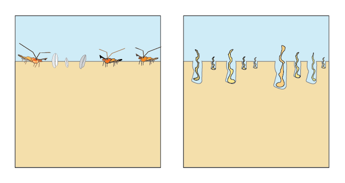
Figure 14.14: Bioturbation is the mixing of solids and porewater in the upper layers by benthic animals. Irrigation causes extra mixing of porewater through their burrows.

Bioturbation is computed to vary with depth below the sediment-water interface, based on selection of an appropriate model, $\Theta_{\text{imix}}^{sdg}$, via the switch imix (equation (14.14), figure 14.15), such that:

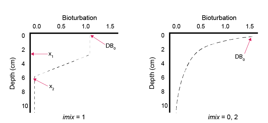
\[\begin{equation} \Theta_{\text{imix}}^{sdg}=\left\{ \begin{array}{@{}ll@{}} 0, & \text{exponential decay curve}\\ 1, & \text{piece-wise two-layer option}\\ 2 & \text{exponential decay curve}\\ \end{array}\right. \end{equation} \tag{14.14}\]

Figure 14.15: Depth profile representing two possible bioturbation options and the functions of the parameters DB0, x1 and x2.

The rate of bioturbation is set with the parameter DB0, whereby the bio-diffusivity is computed as $D_{B}=D_{B}[D_{B_0},z_s]$. If the user selects imix switch 0 or 2, then they use the parameter xs to set the shape of the exponential decay curve. If the user selects imix switch 1, then they use parameters x1 and x2 to set the two depths between which bioturbation goes at the full rate and drops to zero:

imix = 0 Bio-diffusivity:

\[\begin{equation} D_B[z_s] = D_{B_0} e^{-\frac {z_s^2}{2 xs^2}} \end{equation}\]

imix = 1 Bio-diffusivity:

\[\begin{equation} D_B[z_s] =\left\{ \begin{array}{@{}ll@{}} D_{B_0}, & z_s \: \le \: x_1 \\ D_{B_0} \: (\frac {x_2 - z_s} {x_2 - x_1}), & z_s \gt x_1 \text{ and } z_s \le x_2\\ 0 & z_s \gt x_2 \\ \end{array}\right. \end{equation}\]

imix = 2 Bio-diffusivity:

$D_B[z_s] = D_{B_0} \: e^{(- \frac{z_s}{xs} )}$

A bioturbation profile is output in the file Depths.sed, so the user can examine the shape of the profile based on the parameter settings chosen.

Bioirrigation

Bioirrigation has only one option, whereby the parameter alpha0, $\alpha_0$, sets the rate of irrigation and xirrig, $x_{irrig}$, sets the depth at which irrigation decays (equation (14.14), figure 14.16), according to:

alpha Bio-irrigation:

\[\begin{equation} \alpha[z_s] = \left\{ \begin{array}{@{}ll@{}} \alpha_0 , & z_s \: \le \: x_{irrig} \\ \alpha_0 \: e^{-1.5 \: (z_s - x_{irrig})}, & z_s \gt x_{irrig} \\ \end{array}\right. \end{equation} \tag{14.15}\]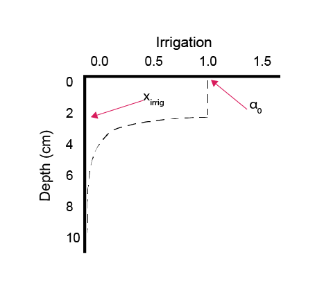

Figure 14.16: Example of a depth profile that sets the rate of irrigation, and the parameters alpha_0 and x_irrig.

Salinity inhibition

A salinity factor, $F_{Sal}$, inhibits processes at hypersaline concentrations. $F_{Sal}$ ranges from 1 to 0, as set between salinity concentration parameters Sal1 and Sal2 (PSU), according to equation (14.16).

\[\begin{equation} F_{Sal} =\left\{ \begin{array}{@{}ll@{}} 1, & Salinity \: \le \: Sal_1 \\ \frac {Sal_2 - Salinity} {Sal_2 - Sal_1}, & Salinity \gt Sal_1 \\ 0 & Salinity \gt Sal_2 \\ \end{array}\right. \tag{14.16} \end{equation}\]

The effect of the scaling is shown in figure 14.17.

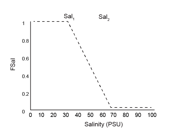
$Diagram of the salinity factor $F_{Sal}$, scaling between 1 and 0 between the parameters. In this diagram `Sal~1~` is 40 and `Sal~2~` is 70.$

Figure 14.17: Diagram of the salinity factor $F_{Sal}$, scaling between 1 and 0 between the parameters. In this diagram Sal~1~ is 40 and Sal~2~ is 70.

$F_{Sal}$ is applied to biota-driven mixing (see below) and to the nitrogen redox and adsorption reactions. It is multiplied by the following reactions:

R_N2O
R_NO2
R_NO3
R_NH4ox
R_NH4NO2
R_NO2O2
NH₄⁺ adsorption

The term affects all rates equally and so does not favour the concentration of any of the species. However, it slows down the transformation of each species into the other, and increased the effect of transport reactions and depth-driven concentration gradients.

H₂S inhibition

High $H_{2}S$ concentration is set to inhibit biota-driven mixing and nitrogen redox reactions, on the basis that $H_{2}S$ is toxic to organisms. An $H_{2}S$ factor, $F_{Sul}$, is an inhibition factor similar to other inhibition factors in the sediment model.

\[\begin{eqnarray} F_{Sul} = \frac {K_{H_{2}S}} {(K_{H_{2}S} + H_{2}S)} \tag{14.17} \end{eqnarray}\]

As with $F_{Sal}$, $F_{Sul}$ scales between 1 and 0, however, as a decay rather than a stepped function (Figure 14.18). The value for KH2S can be found in the physical parameters table below In this simulation, the same value for KH2S was used in all zones.

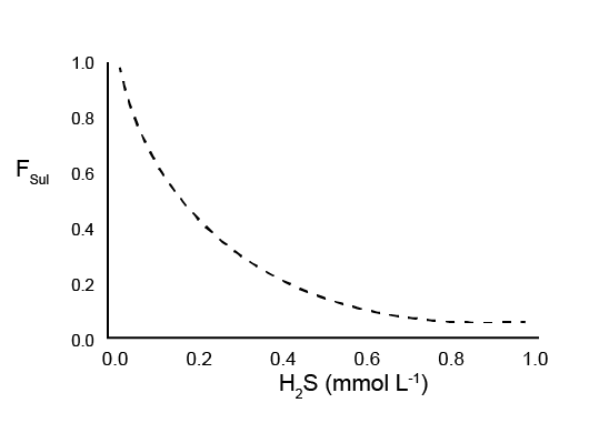
$Diagram of the $H_2S$ factor, $F_{Sul}$, scaling from 1 to 0 as $H_2S$ concentration decreases.$

Figure 14.18: Diagram of the $H_2S$ factor, $F_{Sul}$, scaling from 1 to 0 as $H_2S$ concentration decreases.

Benthic flora

CANDI-AED has two types of benthic plants that can affect $O_2$ concentrations and physical mixing. They have optional links to the water column models.

Microphytobenthos

Microphytobenthos ($MPB$) are small units of phytoplankton that grow on the sediment surface. They are subject to physical transport processes, in the same was as other sediment solids. $MPB$ concentration increases by growing (rather than reacting), which is the difference between its rates of growth (gross primary production, R_gpp) and respiration (R_rsp) (equation (14.18)).

\[\begin{equation} \frac {\delta MPB} {\delta T} = R_{gpp} - R_{rsp} \tag{14.18} \end{equation}\]

R_gpp and R_rsp are calculated according to equations (14.19) and (14.20). MPBdepth and fgpp_sflux are CANDI-AED parameters, set for each zone in the parameters input file. MPBG and MPBR are growth and respiration rate variables linked to the water column model. If they are not present in the water column model, MPBG and MPBR default to zero, which in turn sets R_gpp and R_rsp to zero. From the sediment-water interface down to MPBdepth, the $MPB$ both grow and respire, and below MPBdepth, any $MPB$ that are mixed down to those layers cease to grow, due to a lack of light, but continue to respire at a reduced rate.

\[\begin{equation} R_{gpp} =\left\{ \begin{array}{@{}ll@{}} 0, & depth \: \gt \: MPBdepth \\ \frac{MPBG \times \delta depth} {depth} \times (1 - fgpp - sflux) & depth \le MPBdepth \\ \end{array}\right. \tag{14.19} \end{equation}\] \[\begin{equation} R_{rsp} =\left\{ \begin{array}{@{}ll@{}} \frac {365}{7} \times MPB, & depth \: \gt \: MPBdepth \\ \frac{MPBR \times \delta depth} {depth} \times (1 - fgpp - sflux) & depth \le MPBdepth \\ \end{array}\right. \tag{14.20} \end{equation}\]

R_gpp is a source of $O_2$ in the $O_2$ balance equation. R_rsp consumes $O_2$ and produces organic matter.

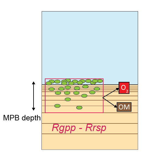
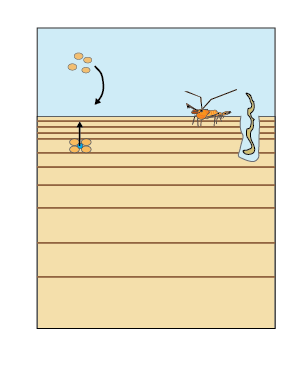
Figure 14.19: Schematic of the parameterisation of $O_2$ injection into the sediment where $MPB$ are respiring.

Aquatic macrophytes

CANDI-AED also includes aquatic macrophytes, such as seagrass or filamentous algae. In a similar way to $MPB$, the roots of macrophtes inject $O_2$ into the upper layers of the sediment. The rate of $O_2$ production, R_rootsO2, is calculated according to (14.21).

\[\begin{equation} R_{RootsO_{2}} =\left\{ \begin{array}{@{}ll@{}} 0, & depth \: \gt \: RTDP \\ \frac {rto2 \times \delta depth}{depth} & depth \le RTDP \\ \end{array}\right. \tag{14.21} \end{equation}\]

The term RTDP is a CANDI-AED parameter, set for each zone. The term rto2 is the $O_2$ excretion rate parameter. It may be sourced from the water column model if the models are linked, or it may be calculated within CANDI-AED if the models are not linked. The options for having the root $O_2$ settins linked or not linked are laid out in table 14.11.

Table 14.11: Macroalgae parameters and variables
CANDI variable	Linking variable or parameter	Description
*Linked: id_mag* > 0**
root	id_rootb	Root density (not used)
rtdp	id_rootd	Root depth
rto2	id_rooto	Root O₂ excretion rate parameter, used in equation
*Not linked: id_mag* = 0**
root	0	Root density (not used)
rtdp	parameter `rootsdepth`	Root depth
rto2	$\displaystyle \ RTO2 = photoo2rate \times (1 - e^{ \frac {-lght} {rootslight} } ) \ $	Root O₂ excretion rate parameter, used in equation
lght	id_par	Light variable from linked model
rootslight	parameter `rootslight`	Light extinction coefficient for root O₂ excretion

The presence of macrophytes also affects the diffusivity at the sediment-water interface. Diffusion is calculated as normal in all layers, but the diffusivity in the top-most layer only is multiplied by the factor swi_deff. swi_deff is calculated according to equation (14.24), where TAUB is the linked variable, and taubsensitivity and smothbm are CANDI-AED parameters, set for each zone. The effect is that when macrophytes are present, they smother the sediment and prevent mixing with the water column.

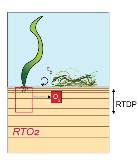
\[\begin{equation} If \ \ \ mag \gt smothbm \\ taub = 0.001 \\ \tag{14.22} \\ \end{equation}\] \[\begin{equation} If \ \ \ mac \gt smothbm \\ taub = 0.001 \\ \tag{14.23} \\ \end{equation}\] \[\begin{equation} swi \text{_} deff = (1.0 + TAUB \times 100) \times taubsensitivity \\ \tag{14.24} \ \\ \end{equation}\]

Figure 14.20: Schematic of macrophyte model: $O_2$ injection into the sediment by seagrass roots and smothering by filamentous algae.

14.3.3 Implementation within the AED framework

While the first part of the model description was about the scientific processes, this second part describes how CANDI-AED functions as one module within the AED framework.

The AED modules are designed to fit together to make a simulation with a desired degree of complexity. Most water quality modules separate reaction processes, and the AED framework is used to combine them. For example, AED Oxygen and AED Organic Matter can be combined with a hydrodynamic model. CANDI-AED is one of the most complex of the modules, in part because it has both reaction and transport components within the module. The processes are not compartmentalised into separate models, and so many switches and parameters are used within CANDI-AED to set the degree of complexity and links to the other modules.

14.3.3.1 Sediment-water coupling

The sediment and hydrodynamic models are coupled at the sediment-water interface. The AED model setup has separate functions for coupling the variables of the bottom-most cell of a hydrodynamic model to the top-most layer of the sediment model:

flux of solid (particulate) material onto the sediment surface, mmol m^-2 d^-1
concentration of dissolved substances in the bottom water, mmol m^-3
flux of dissolved substances from the top sediment layer to or from the water, mmol m^-2 d^-1

Where there is any mismatch between the sediment and water column variables, the factor of part_sed_scale can be used. (part_sed_scale can be found in the file aed_sdg_vars.csv, as outlined in more detail below.) For example, influx of the water column variable $PON$ can be distributed between sediment variables $PON_R$ and $PON_L$. part_sed_scale is a real number between zero and one. For any sediment variables linked to the same water column flux, the part_sed_scale values should sum to 1.

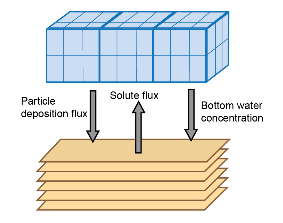
Figure 14.21: Schematic of sediment water coupling interactions

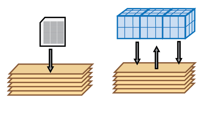
Depending on the nature of the host hydrodynamic model, several configurations can be implemented:

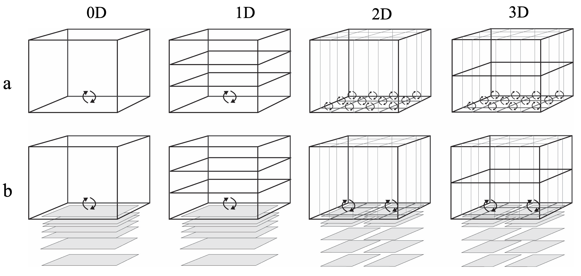
Spatial resolution options available through AED. a) Water column studies have traditionally assigned a flux to the sediment water interface without resolving the sediment chemical concentrations by depth, though they can be resolved laterally. b) The 0D water column is the method used in most sediment diagenesis studies, and use of multiple sediment zones is an option available within AED.

Figure 14.22: Spatial resolution options available through AED. a) Water column studies have traditionally assigned a flux to the sediment water interface without resolving the sediment chemical concentrations by depth, though they can be resolved laterally. b) The 0D water column is the method used in most sediment diagenesis studies, and use of multiple sediment zones is an option available within AED.

Fluxes of dissolved species occur between the sediment and water column. They are calculated from the concentration gradient at the sediment-water interface according to Fick’s Law:

\[\begin{equation} F = D_{0}\frac{\Delta C}{\Delta x} = \frac{D_{0}}{\delta} (C_{bw} - C_{1}) \tag{14.25} \end{equation}\]

where $D_{0}$ is the diffusivity, $\delta$ is the thickness of the diffusive boundary layer at the sediment water interface and defined as the length scale of the first sediment layer, $C_{bw}$ is the bottom water concentration and $C_{1}$ is the concentration in the top sediment layer.

At the bottom of the domain ($x$ = xl) the model can be specified to have a fixed-concentration (deepbc_mode = 0) such that the concentration at $xl = C_{Bot}$, or it can be specified to have a zero-derivative (deepbc_mode = 1) defined as $\frac{dC}{dx}=0$ at $x = xl$.

AED environmental variables can be accessed by CANDI-AED, and in most cases they do not feed back to the water column (see section on environmental variables). Parameter-variables can also be accessed by CANDI-AED, for example taub and w₀₀. taub affects the diffusivity and the sediment-water interface. The deposition rate w₀₀ can be linked to the water column rate using swi_link_variable.

14.3.3.2 Resolving sediment zonation

The sediment model can be set up with multiple zones. The setup is the same as in the description above, and the zone boundares are not necessarily coincident with the grid structure of the water. Using zones is a practical compromise between computational efficiency and capturing spatial heterogeneity in sediment properties and their fluxes.

For a 3D hydrodynamic model, the sediment zones are adjacent areas of the bottom of the domain, for example, stretches of a river from upstream to downstream. A 3D diagram is given in Figure 14.23.

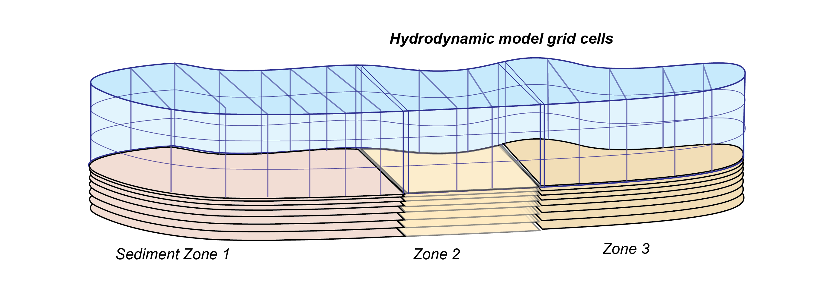
Figure 14.23: Schematic depicting sediment zone numerical approach, for a 3D hydrodynamic mesh.

The equivalent 1D hydrodyanmic model has the water column simulated in vertical layers. The sediment zones are assigned as slices of sediment according to depth. A 1D diagram is given in Figure 14.24.

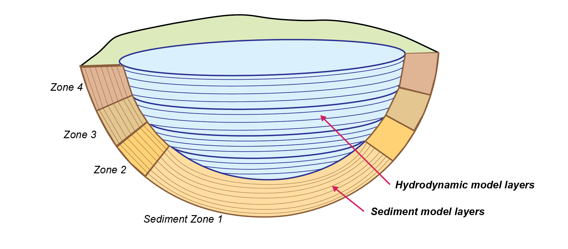
Figure 14.24: Schematic depicting sediment zone numerical approach, for a 1D layered hydrodyanmic model, such as a lake..

The fluxes and concentrations in the water cells above the sediment are averaged for linked variables (Figure (fig:dev-Grid3)).

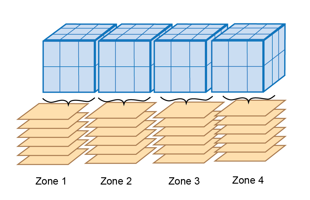
Figure 14.25: Schematic displaying how water cells are averaged when using sediment zones with a 3D hydrodynamic model.

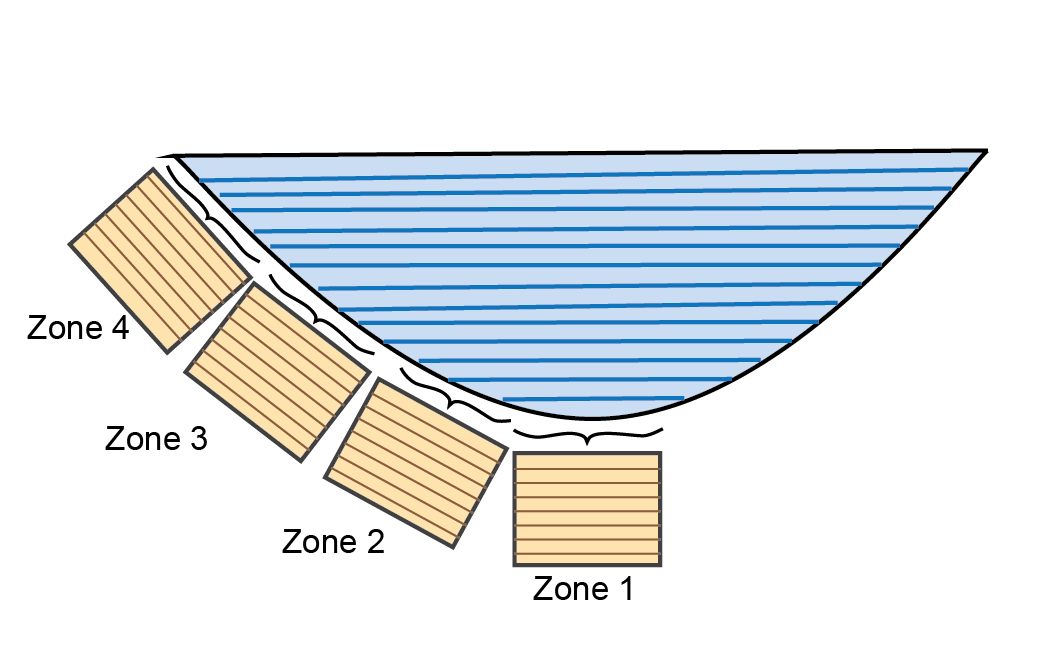
Figure 14.26: Schematic displaying how water cells are averaged when using sediment zones with a 1D hydrodynamic model.

14.3.3.3 Numerical solution

The time-dependent processes in CANDI-AED are solved by an ordinary differential equation solver DVODE. The details of the numerical solution are explained in detail by Boudreau (1997). DVODE was originally developed by Brown et al. (1989) and was used in the predecessors of this code by Boudreau (1996) and Luff et al. (2000).

CANDI-AED sets up the inputs for DVODE as follows:

The boundary conditions are updated at the sediment-water interface and bottom boundary (which may be connected to other modules)

The rates are calculated, for example, as a product of concentration and rate constants, for example,

\[\begin{equation} R_{FeSOx} = k_{FeSOx} [O_2] [FeS] \end{equation}\]
The reactions are calculated, as the sum of the losses or gains from the rates of consumption or production, for example,

\[\begin{equation} \frac {\delta O_2}{\delta t} = - R_{OM} - R_{NH4Ox} + R_{gpp} - R{rsp} + {\ \ } ... \end{equation}\]

The transport is calculated, as the sum of advection, diffusion and biological mixing

For each time step, one numerical matrix is produced, which contains an entry at each depth. In the model code, the matrix is given the simple name y. There is a corresponding matrix, named ydot, which contains all of the changes in the variables between time steps. The matrix y contains:

Dissolved variables
Solid variables
Other variables such as pH, pe, ubalchg and IAPs
Reaction sums
Diffusion
Advection

For example, for the reaction of $O_2$ and $FeS$, the matrix contains a depth entry for concentration of both species. The reaction between them is calculated according to the reaction $R_{FeS}$, which also has an entry at each depth. The $O_2$ is subject to transport processes for solutes, and the $FeS$ for solids. The concentration of the reactants are updated, along with the concentration of products such as $Fe^{2+}$ and $SO_4^{2-}$. This process is then followed for all other species.

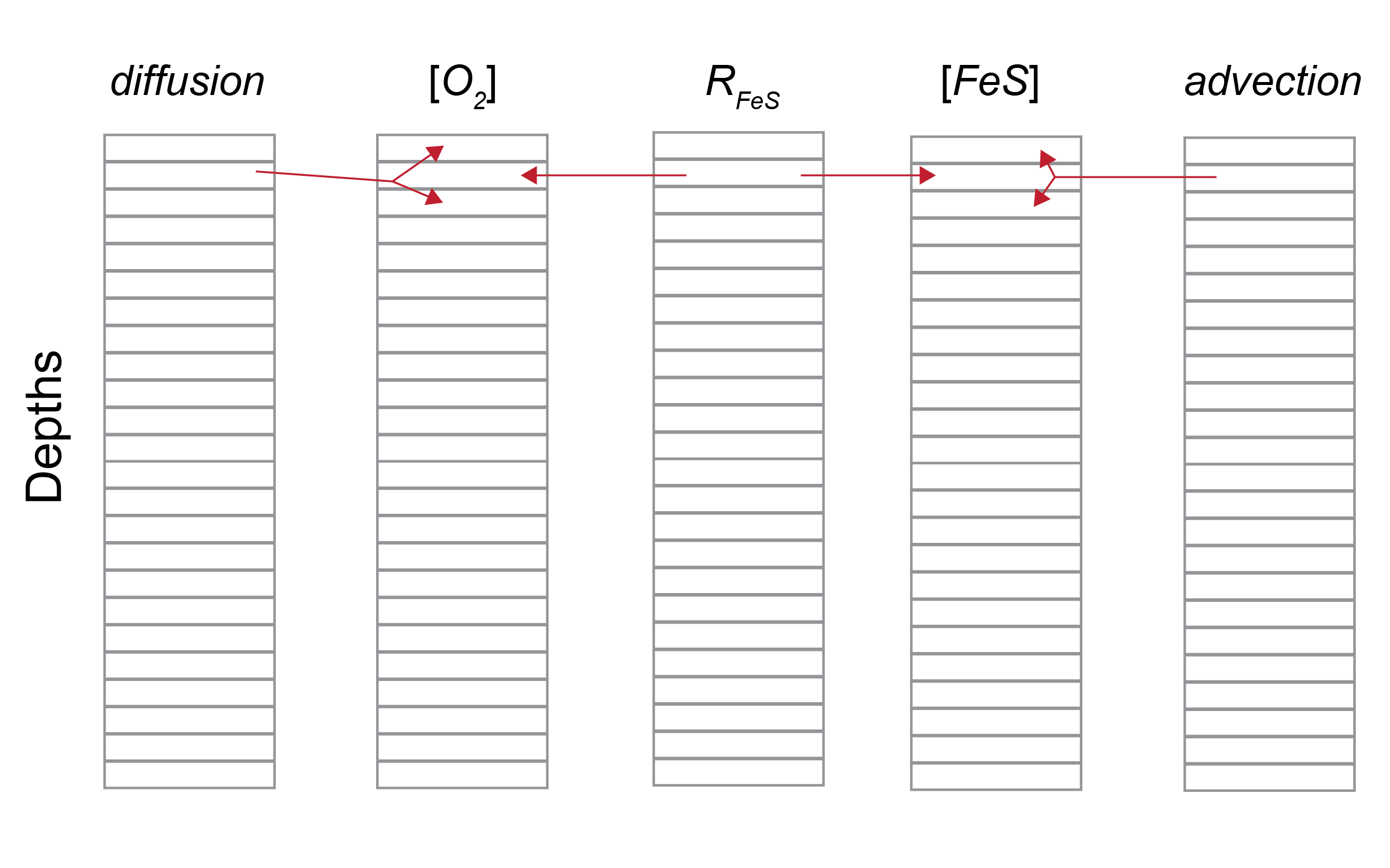
Representation of the matrix structure of the ordinary differential equation solver for and example reaction. With an entry at each depth, the ODE solver calculates the concentrations of reactants from the reactions and transport.

Figure 14.27: Representation of the matrix structure of the ordinary differential equation solver for and example reaction. With an entry at each depth, the ODE solver calculates the concentrations of reactants from the reactions and transport.

14.3.3.3.1 Solute transport equations: subroutine LiqMotion

A subroutine in the model code, named LiqMotion, calculates the solute transport equations. It ultimately produces ydot for solutes, which is used in the difference between time steps. ydot is the sum of diffusion, advection and irrigation, which are calculated separately. They are also calculated differently for each depth layer.

14.3.3.3.1.1 The top layer of the array

14.3.3.3.1.2 The top layer of the sediment

14.3.3.3.1.3 All intermediate layers

14.3.3.3.1.4 The bottom-most layer

14.3.3.3.2 Solid transport equations: subroutine SolMotion

14.3.3.3.2.1 The top layer of the array

14.3.3.3.2.2 The top layer of the sediment

14.3.3.3.2.3 All intermediate layers

14.3.3.3.2.4 The bottom-most layer

14.3.3.4 Module program structure

The sediment diagenesis model CANDI-AED can be used within the AED framework in various ways. This includes a) how the SDG module links to other modules in simulating water variables, and b) how the module operates within the simulated domain.

The general structure of the program is shown in Figure 14.28. The program is firstly initialised (including spin-up days if desired), then loops through the kinetic and equilibrium reactions for each time step and writes the resulting concentrations and rates at each depth to an output file. The kinetic reactions are solved by the VODE program (Brown et al. 1989) and the equilibrium reactions by the Simplex program.

Candi program workflow. The program is firstly initialised, then loops through the kinetic and equilibrium reactions for each time step and writes the resulting concentrations and rates at each depth to an output file. The kinetic reactions are solved by the VODE program and the equilibrium reactions by the Simplex program.

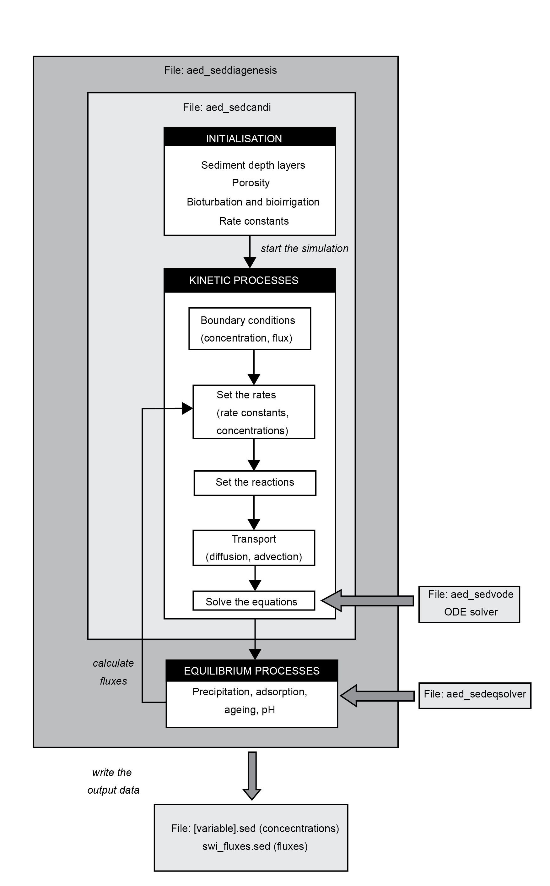
Figure 14.28: Candi program workflow. The program is firstly initialised, then loops through the kinetic and equilibrium reactions for each time step and writes the resulting concentrations and rates at each depth to an output file. The kinetic reactions are solved by the VODE program and the equilibrium reactions by the Simplex program.

14.3.4 Optional module links

In the hierarchy of AED modules, CANDI-AED lies towards the bottom: CANDI-AED can be dependent on many other modules for boundary conditions, and few other modules are dependent on the results of CANDI-AED. CANDI-AED can be run effectively as a stand-alone model or it can be linked to the AED modules.

As outlined in the section on the sediment-water interface, concentration or solid particle flux at the sediment-water interface can supply the top layer of sediment with the value from the bottom most water column cell. A simulation using CANDI-AED can use the following other modules:

aed_sedflux:
aed_tracer
aed_noncohesive
aed_oxygen: $O_2$ concentration can be linked via OXY_oxy
aed_carbon: $CH_4$ and $DIC$ concentration can be linked via CAR_ch4 and CAR_dic
aed_silica
aed_nitrogen: $NH_4^+$ and $NO_3^-$ concentration can be linked via concentration via NIT_amm and NIT_nit
aed_phosphorus: $PO_4^{3-}$ concentration can be linked via PHS_frp
aed_organic_matter: several solid organic matter fluxes can be linked for carbon, nitrogen and phosphorus. including OGM_poc_swi, OGM_pon_swi, and OGM_pop_swi
aed_phytoplankton: the macroalgae settings in CANDI-AED can be linked to environmental variables calculated in the phytoplankton module
aed_totals:

The environmental variables can be used to set parameters and configurations in CANDI-AED, as outlined in the section below.

14.3.5 Feedbacks to the host model

As mentioned above, there are few other modules that are dependent on the results of CANDI-AED, unless the dissolved fluxes at the sediment-water interface are switched on:

aed_sedflux: the parameter sedflux_model controls the setup of zones and whether the flux is taken from a constant value or from CANDI-AED
aed_tracer
aed_noncohesive
aed_oxygen: $O_2$ flux can be linked via SDF_Fsed_oxy
aed_carbon: $CH_4$ and $DIC$ flux can be linked via SDF_Fsed_ch4 and SDF_Fsed_dic
aed_silica
aed_nitrogen: $NH_4^+$ and $NO_3^-$ fluxes can be linked via SDF_Fsed_amm and SDF_Fsed_nit
aed_phosphorus: $PO_4^{3-}$ flux can be linked via SDF_Fsed_frp
aed_organic_matter: several dissolved organic matter fluxes can be linked for carbon, nitrogen and phosphorus, including SDF_Fsed_doc, SDF_Fsed_don and SDF_Fsed_dop
aed_phytoplankton:
aed_totals:

14.3.6 Variable summary

CANDI-AED contains the largest number of variables of any AED water quality module. This section outlines the state variables and diagnostic variables, including those that are compulsory and optional.

14.3.6.1 State variables

A list of the state variables is given in table 14.12. The compulsory variables are key to the biogeochemical processes in CANDI-AED and there is a switch to stop the model running if they are not requested in the variables input csv. Three variables ($pH$, $pe$ and $ubalchg$) are not requested in the input file but they are always calculated and written to the output files. The non-compulsory variables are optional and if they are not included, the model will be allowed to run. However, the results of the calculations may be unpredictable and it is recommended that unless the user is familiar with this model, the variables be left in.

The organic matter variables are more straightforward in this regard, as the OMModel switch leaves the unused organic matter species unreacted. For example, if OMModel = 1, then $POML$ will be a reactive species and $POCL$ will not react. $POCL$ will still be transported and written to the output file, but its concentration will simply disperse from the initial condition.

Table 14.12: Full list of state variables.
Variables	Description
Compulsory variables
‘oxy’	O₂
‘nit’	NO₃^-
‘amm’	NH₄⁺
‘so4’	SO₄^2-
‘h2s’	H₂S
‘frp’	Reactive dissolved PO₄^3-
‘ch4’	CH₄
‘dic’	∑CO₂
Compulsory variables not requested
‘pe’	Redox potential
‘pH’	pH
‘ubalchg’	Charge balance
Non-compulsory variables
‘salt’	Salinity
‘docl’	Labile DOC
‘docr’	Refractory DOC
‘donl’	Labile DON
‘donr’	Refractory DON
‘dopl’	Labile DOP
‘dopr’	Refractory DOP
‘docs’
‘dons’
‘dops’
‘pocs’	Macroaglage C
‘pons’	Macroaglage N
‘pops’	Macroaglage P
‘pocl’	Labile POC
‘pocr’	Refractory POC
‘ponl’	Labile PON
‘ponr’	Refractory PON
‘popl’	Labile POP
‘popr’	Refractory POP
‘n2o’	N₂O
‘no2’	NO₂
‘n2’	N₂
‘pip’	Adsorbed P
‘pipvr’
‘mno2a’	Amorphous MnO₂
‘mno2b’	Crystalline MnO₂
‘mnco3’
‘feii’	Fe²⁺
‘feoh3a’	Amorphous Fe(OH)₃
‘fes’	FeS
‘fes2’	FeS₂
‘feco3’
‘ca’	Ca²⁺
Environmental linked variable
PRES	Pressure
TEMP	Temperature
SALT	Salinity
LGHT	Light
TAUB	Diffusivity
MPBG	Microphytobenthos growth rate
MPBR	Microphytobenthos respiration rate
ROOT	Macrophyte root density
RTDP	Macrophyte root depth
RTO2	Macrophyte root oxygen excretion

14.3.6.2 Diagnostic variables

There is no exhaustive list of the diagnostic variables in CANDI-AED. As described in the outputs section below, most rates and factors can be written to an output .sed file using the list morevariables.

Another set of sheet variables is calculated within CANDI-AED and written to the netcdf output (table 14.13). In order to set the amount of data written to the netcdf and prevent the creation of excessively large files, the parameter diag_level is used to set the number of diagnostics.

Table 14.13: List of diagnostic variables written to the netcdf.
Diag variable	Description	Unit	Group
diag_level > 0
id_opd	Oxygen penetration depth, where O₂ > 0.1 mmol L^-1	cm	diag_level > 0
id_arpd	Apparent redox potential discontinuity, where H₂S > 0.001 mmol L^-1	cm	diag_level > 0
id_fom	Particulate organic matter flux at the SWI. Sum of POCL, POCR and POCS	mmol C m^-2 d^-1	diag_level > 0
id_bur	Particulate organic matter flux at the bottom boundary	mmol C m^-2 d^-1	diag_level > 0
id_toc	Total organic carbon in the top 15 cm	mmol C m^-2	diag_level > 0
id_tfe	Total iron ’*	mmol Fe m^-2	diag_level > 0
id_tn	Total nitrogen in the top 15 cm	mmol N m^-2	diag_level > 0
id_tp	Total phosphorus in the top 15 cm	mmol P m^-2	diag_level > 0
id_ts	Total sulfur ’*	mmol S m^-2	diag_level > 0
id_crs	Chromium reducable sulfur ’*	mmol S m^-2	diag_level > 0
diag_level > 1
id_mnrl	0		diag_level > 1
id_aerb	0		diag_level > 1
id_anrb	0		diag_level > 1
id_dnit	0		diag_level > 1
id_mred	0		diag_level > 1
id_fred	0		diag_level > 1
id_sred	0		diag_level > 1
id_meth	0		diag_level > 1
id_bpp	Net MPB productivity, growth rate minus respiration rate	mmol m^-2 d ^-1	diag_level > 1
diag_level > 2
id_biod	Bioturbation penetration depth, where bioturbation > 2E-5	cm	diag_level > 2
id_poro	Mean porosity	m³ water m^-3 space	diag_level > 2
diag_level > 9
id_stdi	0		diag_level > 9
id_eror	0		diag_level > 9
id_c_swi	Net carbon flux over the sediment-water interface	mmol C m^-2 d^-1	diag_level > 9
id_n_swi	Net nitrogen flux over the sediment-water interface	mmol N m^-2 d^-1	diag_level > 9
id_p_swi	Net phosphorus flux over the sediment-water interface	mmol P m^-2 d^-1	diag_level > 9
id_tnchk	Net nitrogen mass change	mmol N m^-2 d^-1	diag_level > 9
			diag_level > 9

14.3.6.3 Environmental variables

There are several ‘environmental’ variables, that can be linked from the water column model or other AED modules, to set conditions in the sediment model (table 14.14). For example, the set of $MPB$ and $MAG$ variables is used to set the $O_2$ penetration into the upper sediment. Another example is that water column salinity from a model such as TUFLOW-FV can be used to set the sediment-water interface concentration of salt at the sediment-water interface, which is used to calculate F_Sal. Salinity is set as a permanently linked variable from the water column AED model, without using water_link.

Water column salinity is also used to set the boundary concentration of sulfate. Although most dissolved variables are simulated using mmol L^-1, salinity uses practical salinity units (PSU). PSU has a standard concentration of solutes, primarily chloride, sodium, magnesium and sulfate. One PSU correlates to approximately 0.9 mmol L^-1 sulfate, and so the CANDI-AED $SO_4^{2-}$ boundary is fixed at 0.9 $\times$ salinity.

Table 14.14: List of environmental variables.
CANDI variable	Linked variable	Conversion	Description
PRES	id_depth	$\displaystyle \times 1.025E-3$	Pressure
TEMP	id_temp		Temperature
SALT	id_salt		Salinity
LGHT	id_par		Light
TAUB	id_taub		Diffusivity
MPBG	id_mpbg	$\displaystyle \times \frac {1000 \times 365.25}{100 \times 100}$	Microphytobenthos growth rate
MPBR	id_mpbr	$\displaystyle \times \frac {1000 \times 365.25}{100 \times 100}$	Microphytobenthos respiration rate
ROOT	id_rootb		Macrophyte root density
RTDP	id_rootd	$\displaystyle \times \frac {1} {100}$	Macrophyte root depth
RTO2	id_rooto	$\displaystyle \times \frac {1000 \times 365.25}{100 \times 100}$	Macrophyte root oxygen excretion

14.3.7 Parameter and option summary

The preceding details were an explanation of the scientific aspects of this diagenesis model. Practical implementation is outlined below.

The model is set up via the name list text file aed.nml using the module keyword &aed_seddiagenesis and a model namelist block termed &aed_sediment configured to select the sediment_model as “Dynamic” or “Dynamic2D” option. Once this is selected, the model will search for the &aed_sedcandi parameter block.

In addition to adding the code block to aed.nml, users must also supply a valid AED sediment parameter database file (aed_candi_pars.csv is the default name) and a variable definition file (aed_sdg_vars.csv is the default name). If external boundaries are required, then a swibc_file and a deepbc_file also need to be supplied. The four key places for the model setup are summarised in table 14.15), along with the file locations, and whether the settings are different for a simulation with more than one zone.

Users can create a standard file in the correct format from the online AED parameter database by selecting from the available sediment types of interest, downloading via the “Make CSV” button, and then tailoring to the simulation being undertaken as required.

Table 14.15: File locations for major inputs of parameters, initial conditions and boundary conditions.
.	Module level	Zone-specific
Initial condition	InitMethod	Concentrations in
	Organic matter initial profiles parameters	aed_sdg_vars.csv
	.
SWI boundary	default_vals	Variables and zones can be specified in
	water_link	aed_sediment_swibc.dat
	diss_flux_link
	part_sed_link in
	aed_sdg_vars.csv
	.
Bottom boundary	deep_vals in	Variables and zones can be specified in
	aed_sdg_vars.csv	aed_sediment_deepbc.dat
	.
Parameters	Code block in	Majority of parameters in
	aed.nml	aed_candi_params.csv
	&aed_sed_candi
	.

14.3.7.1 Module settings: &aed_sed_candi

The parameters set at the module level are outlined in table 14.16. These parameters are the same for all zones.

Table 14.16: Parameters in &aed_sed_candi.
Parameter	Description	Example value
Timing parameters
spinup_days	Duration of spinup before flux (d)	1
driver_dt	Hydrodynamic model time step (s)	900
substep	Sediment model substep (h)	8
Zone setup parameters
n_zones	Number of zones to simulate. Zones are listed in `active_zones` (integer)	5
active_zones	Sequence of zones to be simulated (integer)	1,3,4,6,7,8,30,31
zone_types	Type of zone, as listed by header in aed_sdg_vars.csv (integer)	1,1,1,1,1,1,1,1,1,1,1,1,1,1,1,1
External parameter file paths
dbase	External candi parameter file path (text)	‘../../external/AED/aed_candi_params.csv’
vars_files		‘../../external/AED/sdg_vars.csv’
geochem_file	External equilibrium chemistry solver parameter file path (text)	‘../../external/AED/aed_geochem_pars.dat’
Boundary condition parameters and files
swibc_mode	Sediment-water interface boundary switch	0
deepbc_mode	Bottom boundary switch	1
swibc_file	Sediment-water interface boundary file path (text)	../../external/AED/aed_sediment_swibc.dat’
deepbc_file	Deep boundary file path (text)	../../external/AED/aed_sediment_deepbc.dat’
swibc_filevars	Variables taken from external boundary file for sediment-water interface	‘oxy’,‘nit’,‘amm’,‘frp’,‘poml’
deepbc_filevars	0	‘poml’
Initial condition setup
SolidInitialUnit		‘mmolLsolid’
OMInitMethodL	Switch for labile organic matter initial profile (constant, linear or exponential) (character switch)	‘LI_I’
OM_topL	Fraction of initial condition at the top of the labile initial profile using linear option (0 to 1)	1
OM_minL	Fraction of initial condition at the depth InitMinDepthL using linear option (0 to 1)	0.9
OM_cfL	Decay coefficient for labile organic matter initial profile using exponential option (-)	0.6
InitMinDepthL	Depth at which the OM_minL percentage applies using the linear option (cm)	99
OMInitMethodR	Switch for refractory organic matter initial profile (constant, linear or exponential) (character switch)	‘LI_I’
OM_topR	Fraction of initial condition at the top of the refractory initial profile using linear option (0 to 1)	1
OM_minR	Fraction of initial condition at the depth InitMinDepthR using linear option (0 to 1)	0.9
OM_cfR	Decay coefficient for labile organic matter initial profile using exponential option (-)	0.6
InitMinDepthR	Depth at which the OM_minR percentage applies using the linear option (cm)	99
POMVR	Concentration of very refractory particulate organic matter (% solids)	0.3
Output settings
diag_level	Switch for which types of diags to write to files (integer)	10
output_profiles	Switch to write .sed files (logical)	.TRUE.
morevariables	List of other variables to be written to output files e.g. rates, factors etc. (text)	‘FO2’
output_diag_vars	List of variables to be written to diag files at `output_diag_depths` (text)	‘oxy’,‘amm’,‘poml’
n_ddpths	Number of depths to write diag outputs for. Depths are listed in `output_diag_depths` (integer)	1
output_diag_depths	Depths to write diag files (cm)	1

14.3.7.2 Zone-specific parameters

The majority of CANDI-AED parameters are specified for each zone, using the input parameter file. The default name is aed_candi_pars.csv but the user can change this in aed.nml &aed_sedcandi.

Physical domain and numerical parameters

The physical properties of the sediment are given in Table 14.17 and 14.18. In general, the SDG module was set to run with a time-step of 2 hours, resolve a vertical sediment depth of 80 cm using 50 layers.

Some parameters are set as constant values for all zones, while others are set to be variable in each zone. The variability of bioturbation and irrigation along the length of the lagoon is set using the depth of the effect ($x_1$, $x_2$ and $x_{irrig}$) rather than the intensity ($DB_0$, $\alpha_0$). Upper porosity $\rho_0$ is held at 0.9 (i.e. 90% porewater) for all zones and the lower porosity $\rho_{00}$ is based on measured data at sites in each zone.

Table 14.17: Sediment physical properties, given in aed_candi_parameters.csv.
Parameter	Description	Example value
p0	Upper porosity (-)	0.90
p00	Lower porosity (-)	0.39
taubsensitivity	Diffusion sensitivity to external transport (-)	1.00
w00	Sediment accumulation rate (cm y^-1)	1.00
db0	Bioturbation rate (cm^-2 y^-1)	40.00
poreflux	Porewater advection rate (cm y^-1)	0.00
Sal1	Lower salinity concenration for F_Sal (PSU)	35.00
Sal2	Upper salinity concenration for F_Sal (PSU)	70.00
kH2S	H₂S concentration for K_Sul (mmol L^-1)	0.10
swibc_mode	Sediment-water interface boundary switch	0.00
deepbc_mode	Bottom boundary switch	1.00

Table 14.18: Sediment layer setup parameters and mixing parameters that might vary by zone, to set simulation with differences in sediment quality across space, given in aed_candi_parameters.csv.
Parameter	Description	11	12	…
p0	Upper porosity (-)	0.90	0.90	…
p00	Lower porosity (-)	0.39	0.39	…
xl	Simulation depth	80.00	80.00	…
maxnpts	Number of sediment layers	50.00	50.00	…
job	Switch for linear or exponential layer spacing	2.00	2.00	…
x1	Depth of full bioturbation (cm)	0.50	0.50	…
x2	Depth of bioturbation decline (cm)	1.00	1.00	…
alpha0	Irrigation rate (cm y^-1)	200.00	200.00	…
xirrig	Depth of irrigation (cm)	1.00	1.00	…

Organic matter parameters

Many of the key processes in the sediment are driven by organic matter oxidation. Fresh organic matter supplied to the sediment surface fuels the bacterially-driven primary redox reactions that constantly shift the chemical equilibrium in the sediment. Organic matter metabolism also releases organic N and P to the water column. The parameters are given in Table 14.19.

The organic matter model option number 2 was used in this project. This option has both particulate and dissolved organic phases, and simulates organic C, N and P as separate state variables.

Table 14.19: Organic matter oxidation parameters, given in aed_candi_parameters.csv.
Parameter	Description	Example value
OMModel	Complexity of OM model	2.0e+00
OMapproach	Limitation function switch	1.0e+00
docl2dic	Description	1.0e+02
donl2din	Labile DON terminal metabolism rate (y^-1)	1.0e+02
dopl2dip	Description	1.0e+02
pocl2docl	Labile POC hydrolysis rate (y^-1)	5.0e+01
ponl2donl	Description	5.0e+01
popl2dopl	Labile POP hydrolysis rate (y^-1)	5.0e+01
docr2docl	Description	2.5e+00
donr2donl	Refractory DON terminal metabolism rate (y^-1)	2.5e+00
dopr2dopl	Description	2.5e+00
pocr2docr	Refractory POC hydrolysis rate (y^-1)	5.0e+00
ponr2donr	Description	5.0e+00
popr2dopr	Refractory POP hydrolysis rate (y^-1)	5.0e+00
pocvr2docr	Description	0.0e+00
ponvr2donr	Very refractory PON hydrolysis rate (y^-1)	0.0e+00
popvr2dopr	Description	0.0e+00
domr2dic	Refractory DOM terminal metabolism (y^-1)	1.0e-02
domr2pomr	Description	1.0e-03
poml2doml	Labile POM hydrolysis (y^-1)	1.0e+00
pocu	Description	1.0e+06
ponu	Minimum concentration of refractory PON at which reactions stop (mmol L^-1)	5.0e+03
popu	Description	1.0e+04

Secondary redox reactions

Secondary redox reactions are formed from the by-products of primary redox reactions. The nitrogen redox cycle parameters are given in Table 14.20.

Table 14.20: Nitrogen redox cycle parameters, given in aed_candi_parameters.csv.
Parameter name	Description	Example value
kin_denitrit	Inhibition concentration of denitritation (mmol L^-1)	0.000297
kpart_ammox	Inhibition concentration of ammonium oxidation (mmol L^-1)	0.001000
kin_denitrous	Inhibition concentration of denitrousation (mmol L^-1)	0.000205
kin_deamm	Inhibition concentration of deammonification (mmol L^-1)	0.000886
klim_denitrat	Limitation concentration of denitratation (mmol L^-1)	0.001000
kpart_denitrit	Partitioning concentration of denitritation (mmol L^-1)	0.006000
knh4no2	NH_$⁺ oxidation by NO₂^- kinetic rate (mmol^-1 L y^-1)	0.365000
kno2o2	NO₂ oxidation kinetic rate (mmol^-1 L y^-1)	0.001000

Secondary redox parameters for other processes are given in Table 14.21.

Table 14.21: Secondary redox parameters, given in aed_candi_parameters.csv.
Parameter	Description	Example value
kMnFe	Fe²⁺ oxidation by MnO₂ rate (mmol^-1 L y^-1)	3.0e+03
kTSMn	H₂S oxidation by MnO₂ rate (mmol^-1 L y^-1)	2.0e+01
kTSOX	H₂S oxidation rate (mmol^-1 L y^-1)	1.6e+02
kTSFe	H₂S oxidation by Fe(OH)₃ rate (mmol^-1 L y^-1)	8.0e+00
kPyrite	FeS₂ precipitation rate (mmol^-1 L y^-1)	2.3e-04
kMnFe	Fe²⁺ oxidation by MnO₂ rate (mmol^-1 L y^-1)	3.0e+03
kTSMn	H₂S oxidation by MnO₂ rate (mmol^-1 L y^-1)	2.0e+01
kCH4OX	CH₄ oxidation rate (mmol^-1 L y^-1)	1.0e+07
kCH4SO4	CH₄ oxidation by SO₄^2- rate (mmol^-1 L y^-1)	1.0e+00

Geochemistry parameters

Equilibrium and precipitation/dissolution constants are given in Table 14.22.

Table 14.22: Geochemistry and precipitation/dissolution parameters, given in aed_candi_parameters.csv.
Parameter	Description	Example value
rxn_mode	Geochemical reaction complexity	0
ads_use_pH	Use of pH in adsorption reactions	.true.
PO4AdsorptionModel	Switch for PO₄^3- adsorption options (integer)	1
KPO4p	PO₄^3- adsorption constant for PO4AdsoprtionModel = 1 (-)	1.05
NH4AdsorptionModel	NH₄⁺ adsorption model switch	1
kPyrite	FeS₂ precipitation rate (mmol^-1 L y^-1)	2.3000000000000001E-4
kFeSppt	FeS precipitation kinetic rate	1E-3
kFeSdis	FeS dissolution kinetic rate	1E-3
KPFeS	Equilibrium constant for FeS precipitation (-)	-2.2000000000000002

Hidden parameters: aed_readcandi.F90

A set of parameters that the user is unlikely to need to change has been removed from the model input files and set in the model code (table 14.23).

Table 14.23: Other parameters, which are not currently listed in the parameter input file.
Parameter	…2
w00_min
w00_max
w00_link_scale
SolidInitialUnit
theta_om
kpo2n2o
Temporary_proton
knh4ox_to_N2O
dG0ManH2
YManH2
klim_denitrit
kpNO2
kpN2O
kpO2NO3
kpO2NO2
lNO2
lpNO2
lN2O
lpN2O
lpo2no2
lpo2n2o
KNH4p
DOMAdsorptionModel
KDOMp
kmn
kpmn
kfe
kpfe
lmn
lpmn
lfe
lpfe
kanh4
kapo4
fgpp_sflux
Xgpp_n
Xgpp_p
Xrsp_n
Xrsp_p
Xrsp_co2
Xrsp_doc
Xrsp_poc
smothbm

14.4 Setup & Configuration

An example aed.nml configuration block for the aed_seddiagenesis module that includes multiple active sediment zones, plus microphytobenthos (MPB) and seagrass links, is shown below:

!###############################################################################
! aed_seddiagenesis
!-------------------------------------------------------------------------------
&aed_sediment
   sediment_model    = 'DYNAMIC'    ! engages the CANDI-AED model
   mpb_link_variable = 'PHY_mpb'    ! use to set link for MPB
   mag_link_variable = 'MA2_mag'    ! use to set link for macroalgae inputs
   mac_link_variable = 'MAC_mac'    ! use to set link for macrophyte root inputs
   swi_link_variable = 'NCS_swi'    ! use to set link for variable w00
/
&aed_sed_candi
  !-- Time Settings --!
   spinup_days     =  90
   spinup_dt       =   0.25
   driver_dt       = 900     
   substep         =   8       
  !-- Zones details --!
   n_zones         = 5
   active_zones    = 104,103, 53, 23, 12,11
   zone_types      =   5, 3, 3, 1, 1
  !-- General Setup Options  --!
   dbase           = './AED/aed_candi_params.csv'
   vars_files      = './AED/aed_sdg_vars.csv'
   geochem_file    = './AED/aed_geochem_pars.dat'
  !-- Sediment Boundary Conditions  --!
   swibc_mode      = 0      ! previously ibc2
   deepbc_mode     = 1      ! previously ibbc
   swibc_file      = './AED/aed_sediment_swibc.dat'
   deepbc_file     = './AED/aed_sediment_deepbc.dat'
   swibc_filevars  = '' ! 'oxy', 'nit', 'amm', 'frp', 'poml'   ! from_bc_file
   deepbc_filevars = '' ! ,OXY_oxy,                            ! use_deep_bc
   flux_scale      = 1
  !-- Initial Conditions  --!
   SolidInitialUnit= 'mmolLsolid'
   OMInitMethodL   = 'LI_I'
   OM_topL         = 1
   OM_minL         = 0.9
   OM_cfL          = 0.6
   InitMinDepthL   = 99
   OMInitMethodR   = 'LI_I'
   OM_topR         = 1
   OM_minR         = 0.3
   OM_cfR          = 0.6
   InitMinDepthR   = 50
   POMVR           = 0.3
  !-- Outputs  --!
   diag_level         = 10
   output_profiles    =  .TRUE.
   morevariables      = 'Rgpp','Rrsp','FO2','f_an'
   output_diag_vars   = 'mpb','oxy','amm','docl','pocl','docr'
   n_ddpths           = 2
   output_diag_depths = 1.0, 5.0  ! cm below swi
/

In addition to adding the above code block to aed.nml, users must also supply a valid AED sediment parameter database file (aed_candi_pars) and a variable definition file (‘aed_sdg_vars’). Both of these files file must be supplied in either CSV format. Users can create a standard file in the correct format from the online AED parameter database by selecting from the available sediment types of interest, downloading via the “Make CSV” button, and then tailoring to the simulation being undertaken as required. Carefully check the parameter units and values!

The sections above described the scientific and technical processes within the model, the links to other AED modules, and the range of variables and parameters. This section outlines how the model treats the initial condition and boundary conditions.

14.4.1 Setup details and examples

This section contains a set of steps for how to set up a simple simulation. Due to the large number of variables and parameters in CANDI-AED a full set of example parameters is not presented here. However, the lists of the tables above all contain example values that the user can consult.

14.4.1.1 Hydrodynamic model setup details and examples

The duration of the sediment model simulation is set within the parameters of the hydrodynamic driver model. For example, if using GLM, the duration is set in glm.nml, &time, then either if timefmt = 2, the start and stop times are set, or if timefmt = 3, the num_days parameter sets the number of days. If using TUFLOW-FV, the time is set in the .fvc file, where the start time and stop time are set as dates.

The sediment zone setup of the hydrodynamic model is also set in the hydrodynamic model parameters. The sediment model can be run without any zones, however, if zones are required, the user will need to make sure the zone numbers are aligned.

14.4.1.2 Module settings and examples

Recommendations for the module-level settings, and information about the necessary modules that are related to CANDI-AED are given below. Please see the parameter section above for the full list of names, units and examples of the module-level parameters.

&aed_sed_candi

Most parameters in the &aed_sed_candi block can be left at the default values. The substep and driver_dt can be adjusted to optimise the simulation for speed and numerical stability. If the simulation is stable, then spinup_days are not required. The list of active_zones should correspond to the zones set in the hydrodynamic model and the parameter files. Users should check that the file paths and file names of the parameter and variable files are correctly set up in the user’s directories. The boundary condition parameters and the initial condition parameters can be left at their default values. From the output settings, the output_profiles can be set to TRUE so that the .sed files are written. Any morevariables and output_diag_vars are set here.

&aed_models

The user should ensure that aed_seddiagenesis is included in the models list. It must come after aed_totals.

&aed_sedflux

The parameter sedflux_model must be set to Dynamic2d for the sediment-water column models to be coupled.

&aed_sed_const2d

If the sediment model is running in fewer zones than the water column model, then the water column model takes constant values for the sediment fluxes. The fluxes are listed in this code block.

&aed_sediment

Some of the names of the linking variables are listed here, for example, mpb_link_variable = PHY_mpb, mag_link_variable = MA2_mag, mac_link_variable = MAC_mac and swi_link_variable = NCS_swi.

Fsed linking variables

The names of Fsed linking variables are set in the various nml blocks. If a linking flux is desired, the user should check that each linking variable is set properly in each block. For example, to link the diss_flux_link for $O_2$, the parameter Fsed_oxy_variable is set to SDF_Fsed_oxy in aed_oxygen and also in the variables .csv file. This applies similarly for &aed_nitogen Fsed_amm_variable = SDF_Fsed_amm and SDF_Fsed_nit.

14.4.1.3 Zone-specific parameter details and examples

Recommendations for the zone-level settings are given below. All parameters can be set for each zone and therefore used to configure zones differently. If only one zone is needed, then the first set of parameters are used. Please see the parameter section above for the full list of names, units and examples of the zone-level parameters.

Physical domain and numerical parameters

The parameters xl and maxnpts set the depth of the simulation and the number of layers. xl is often set to around 30 cm. This is deeper than biological mixing and it is around the depth of a field measurement such as a grab sample or core. Deeper than around 50 cm, most diagenetic processes are stable compared to the upper layers and so it is unlikely that a simulation deeper than 50 is necessary. The number of layers, maxnpts can be around 50. The simulation will require enough layers to resolve a profile of the upper sediment layers and few enough layers to keep the output file size to a minimum. Some tuning of maxnpts may be necessary if the simulation is unstable.

The porosity parameters p0 and p00 are key parameters that can make a simulation specific to a study site. For example, a sandy sediment can have low porosity whereas a clay sediment can have very high porosity. Similarly, the sedimentation rate w00 has a large effect on the dynamics of a simulation and it is an important parameter for making a simulation specific to a study site. Unfortunately, it is rarely measured in the environment.

Bioturbation and bioirrigation depths (x1, x2 and xirrig) have a large effect on the evolution of concentration profiles. If the water column is well oxygenated then these parameters will influence the oxic depth. These parameters also reflect a study site. If an environment has a healthy benthic environment, there will be a lot of mixing, whereas a eutrophic, hypersaline or anoxic environment will have little or no mixing.

Organic matter parameters

The OMModel parameter is used to set the complexity of the organic matter setup. The simplest is OMModel = 1, which can also be most easily compared with published studies. Once the OMModel is set, the oxidation rate parameters are set. For example, for OMModel 1, the oxidation rates of the labile and refractory phases can be set to approximately poml2dic = 100 and pomr2dic = 1 y^-1. (A literature survey of this parameter can be found in Paraska et al. 2014.)

Secondary redox parameters

Default parameters can be used for nitrogen redox parameters, unless a simulation is specifically trying to tune to concentrations of nitrogen redox species. Other secondary redox parameters can be left at the default settings.

Geochemistry parameters

The key geochemistry paramter to select is rxn_mode (see section Mineral precipitation and ageing and 14.10 above). rxn_mode = 0 turns off precipitation, ageing and pH and is therefore the simplest setup. rxn_mode = 2 allows the constant precipitation and ageing of minerals, without any equilibrium.

14.4.1.4 Boundary setting details and examples

Sediment-water interface boundary

Boundary condition settings are described below in the Boundary settings section, including example fluxes and concentrations. The simplest boundary setting is default_vals rather than linked variables or the boundary file. In general, oxidised variables are present at the sediment-water interface, for example, $O_2$, $NO_3^-$, $MnO_2$ and $Fe(OH)_{3A}$. (Reduced species can be used in the initial profiles.) $SO_4^{2-}$ is generally at the sediment-water interface in a saline environment and not in a freshwater environment.

14.4.1.5 Initial condition setup details and examples

Initial condition settings are described below in the Sediment initialisation options section, including examples of concentrations (of solids or in porewater). The simplest setup can start with low or zero concentrations and allow the profiles to evolve. In general, reduced species will be present in the sediment, for example $NH_4^+$, $Mn^{2+}$, $Fe^{2+}$, $H_2S$ and $CH_4$. The exact concentrations can be set for each variable according to any available measured data.

14.4.2 Sediment initialisation options

Before the first time step starts, CANDI-AED loads in an initial concentration profile for each state variable. There is also a period of ‘negative time’ before the full reactive transport system begins.

Initialisation of concentration profiles

Concentration profiles are set using one of five options (figure 14.29):

constant, I_CON
exponential decrease, I_EXP
linear, concentrated at the sediment-water interface, I_SWI
linear, concentrated at depth, I_DEP
a spike, I_SPK

The user sets the initial concentration, a depth where it changes InitMinDepth and a proportion (0 to 1) of the initial concentration _Min.

The constant option as a constant concentration from the sediment-water interface to the deepest layer. This is the default for most variables if no other parameters are set.

The exponential option as the initial concentration at the sediment-water interface and an exponential decay to the bottom of the sediment. This is the default for most labile organic matter species.

The first linear option has the initial concentration at the sediment-water interface and a linear decrease in concentration to the InitMinDepth, where the concentration is the _Min parameter multiplied by the initial concentration. This is the default for most refractory organic matter species, as wel as $FeOH_A$ andd $MnO_{2A}$.

The other linear option has the initial concentration at the InitMinDepth, and the a linear increase in concentration to the sediment-water interface, where the concentration is the _Min parameter multiplied by the initial concentration. This is the default for $NH_4^+$ and $Fe^{2+}$.

The spike option has a peak of concentration at the depth InitMinDepth, a linear increase from the sediment-water interface to that depth, and a linear decrease from that depth to 2 $\times$ the InitMinDepth, below which the concentration is zero. The concentration peak is the initial concentration, and the concentration at the sediment-water interface and the deep sediment is the _Min parameter multiplied by the initial concentration. This option is like a combination of I_SWI and I_DEP. Three examples of the spike initial profile are shown below, depending on the depth of InitMinDepth (14.30).

The concentration for each variable is set in the input file aed_sdg_vars.csv, in the column initial_vals (14.31). If the simulation has several zones, then the initial concentration for the zone is set in other columns in the csv, under the column headings initial_01, initial_02 etc. If there is no initial column in the csv for a particular zone, then the zone defaults to the value in the initial_vals column. The parameters for the depth and proportion are set in aed.nml.

Figure 14.29: Schematic of four of the options for initial profiles.

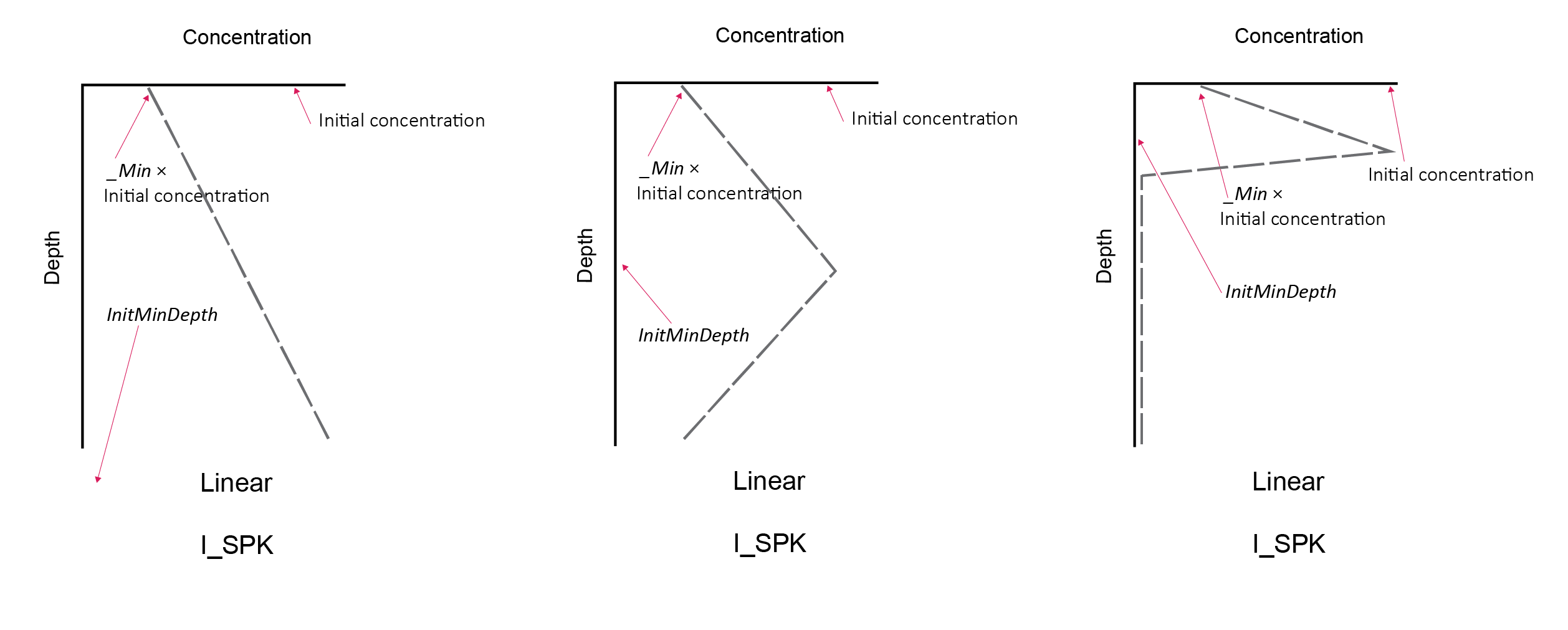
Figure 14.30: Schematic of three possible ways the spike initial profile can appear, depending on the depth parameter InitMinDepth.

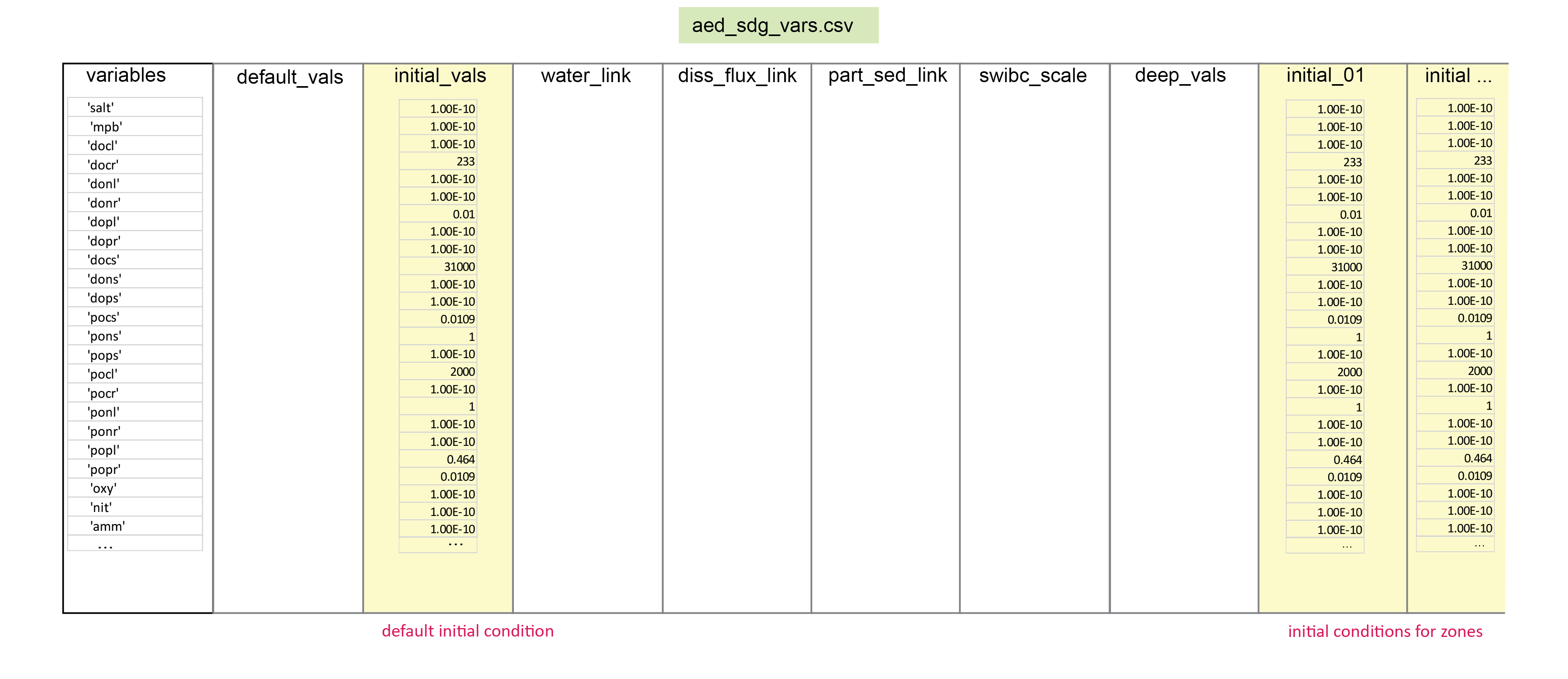
Simplified image of the `aed_sdg_vars.csv` input file. For initialisation, the `variables` need to be set, along with default `initial_vals` or zones-specific `initial_01`, `initial_02` etc. columns.

Figure 14.31: Simplified image of the aed_sdg_vars.csv input file. For initialisation, the variables need to be set, along with default initial_vals or zones-specific initial_01, initial_02 etc. columns.

14.4.2.1 Initialisation of organic matter profiles

For organic matter, the initial profiles are set to either the linear or exponential options. For the linear option, the initial concentration is still taken from initial_vals in aed_sdg_vars.csv. The upper and lower concentrations are set as percentages of the initial concentration using the parameters OM_top and OM_Min, which are found in the &aed_sed_candi block in the aed.nml namelist. There are separate parameters for labile and refractory organic matter, so the parameter names are in fact OM_topL and OM_topR, and OM_minL and OM_minR. These parameters are real numbers as decimals between 0 and 1. The OM_Top fraction applies to the surface concentration. The OM_Min applies at the depth InitMinDepth (cm), which is also set in the &aed_sed_candi block.

For the exponential option, the initial concentration decreases according to equation @ref(eq#init-7b):

\[\begin{eqnarray} concentration = initial vals \times e^ {- OM cfl \times depth} \tag{14.26} \end{eqnarray}\]

The shape of the curve is determined by the parameter OM_cfl, which is found in the &aed_sed_candi block.

14.4.2.2 Timing switches

The duration of the simulation is determined by the hydrodynamic model and its parameter inputs. Other timing parameters are set as outlined below.

Substep

The general task for the reactive transport model is to calculate a change in concentration over time, as a function of a change in concentration over space and as a result of chemical reactions. The general form of this is given in equation (14.27). When this is solved numerically, it is discretised by small increments of time, which are referred to as ‘time steps’ (Δt in equation (14.28)).

To allow the part of the model that solves these differential equations to process a large change in concentration over space or because of a large reaction, the timestep can be multiplied by a substep factor. Examples of where this is needed include a sharp concentration gradient over a small area, or in influx of a large amount of highly reactive substances.

\[\begin{eqnarray} \frac {\delta C} {\delta t} = \frac {\delta C} {\delta x} + reactions \tag{14.27} \\ \\ {\Delta C} = (\frac {\Delta C} {\Delta x} + reactions) \times \Delta t \tag{14.28} \end{eqnarray}\]

Spinup substep

In some simulations the initial timesteps have a high probability that the numerical model may crash while processing the initial condition (figure 14.32). A slow substep overcomes this problem, however, it has the disadvantage of producing a longer run time. The solution for this problem is the tool firststeps (y), which sets an initial time period during which a slower substep (substep_0) is used, and after which the normal substep (substep_1) is used. The switch timeswitch must be set to 1 for this feature to work, otherwise the normal substep applies.

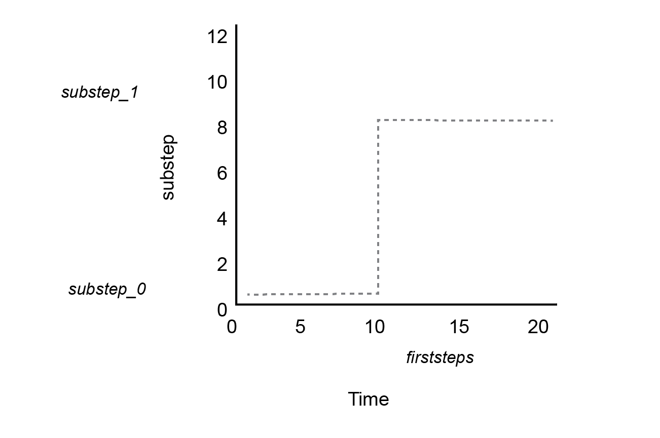
Schematic of the timestep across time. A different timestep (`substep_0`) can be used for a period (`firsteps`) until another timestep is used (`substep_1`).

Figure 14.32: Schematic of the timestep across time. A different timestep (substep_0) can be used for a period (firsteps) until another timestep is used (substep_1).

Transport without reaction

Another tool to help move through the spinup period is to allow transport processes to occur before the reactions start (figure 14.33). This evens out sharp chemical concentration gradients. This allows the simulation to start before the proper time of the simulation, represented in 14.33 as negative time. The parameter spinup_days is the number of timestep integers of negative time, and spinup_dt is the length of each timestep (h). No fluxes at the sediment-water interface occur during negative time.

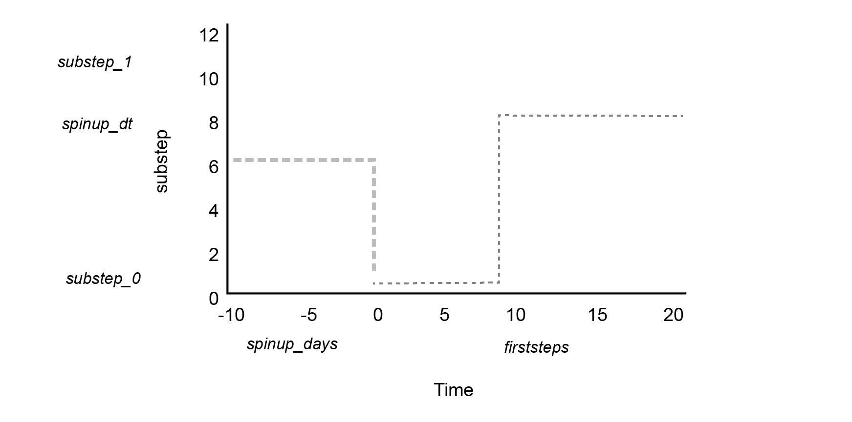
Figure 14.33: Schematic of the timestep over time. The initial period up to spinup_days occurs in ‘negative time’, at a duration of spinup_dt.

Evolution of concentration profiles

After initialisation, the concentration profile develops through the course of the simulation. Some of the most common ways for the profile to develop are given in figure 14.34.

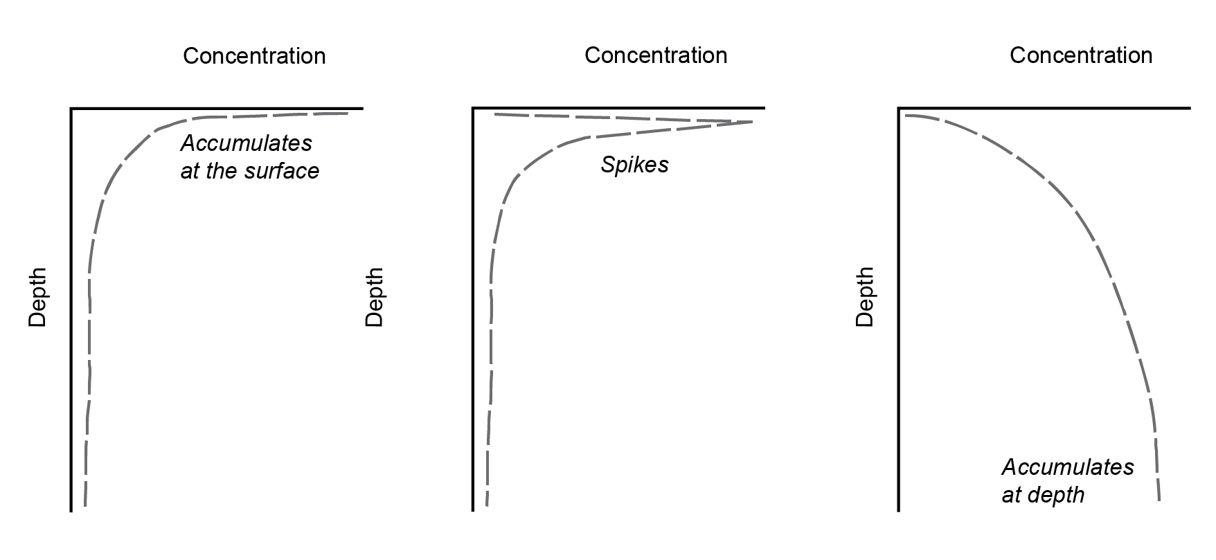
Examples of how the concentration profiles develop after initialisation. Left: the variable accumulates at the surface. Centre: a concentration spike develops. Right: the variable accumulates in the deep sediment.

Figure 14.34: Examples of how the concentration profiles develop after initialisation. Left: the variable accumulates at the surface. Centre: a concentration spike develops. Right: the variable accumulates in the deep sediment.

14.4.3 Boundary settings

Sediment-water interface boundary

Static option: default_vals

For the boundary at the sediment-water interface, the value is set using the default_vals column in the input file aed_sdg_vars.csv (figures 14.35, 14.36). These values are constant in time for the entire simulation. Solids are a deposition flux (mmol m^-2 y^-1) and solutes are a concentration (mmol m^-3). Variables may have other switches or options applied to them, as outlined below, but otherwise the values default to this. To enable this option, set swibc_mode = 1.

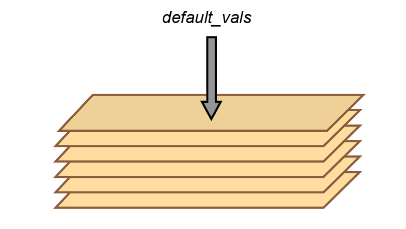
Figure 14.35: Sediment-water interface boundary inputs that are constant in time are set with default_vals.

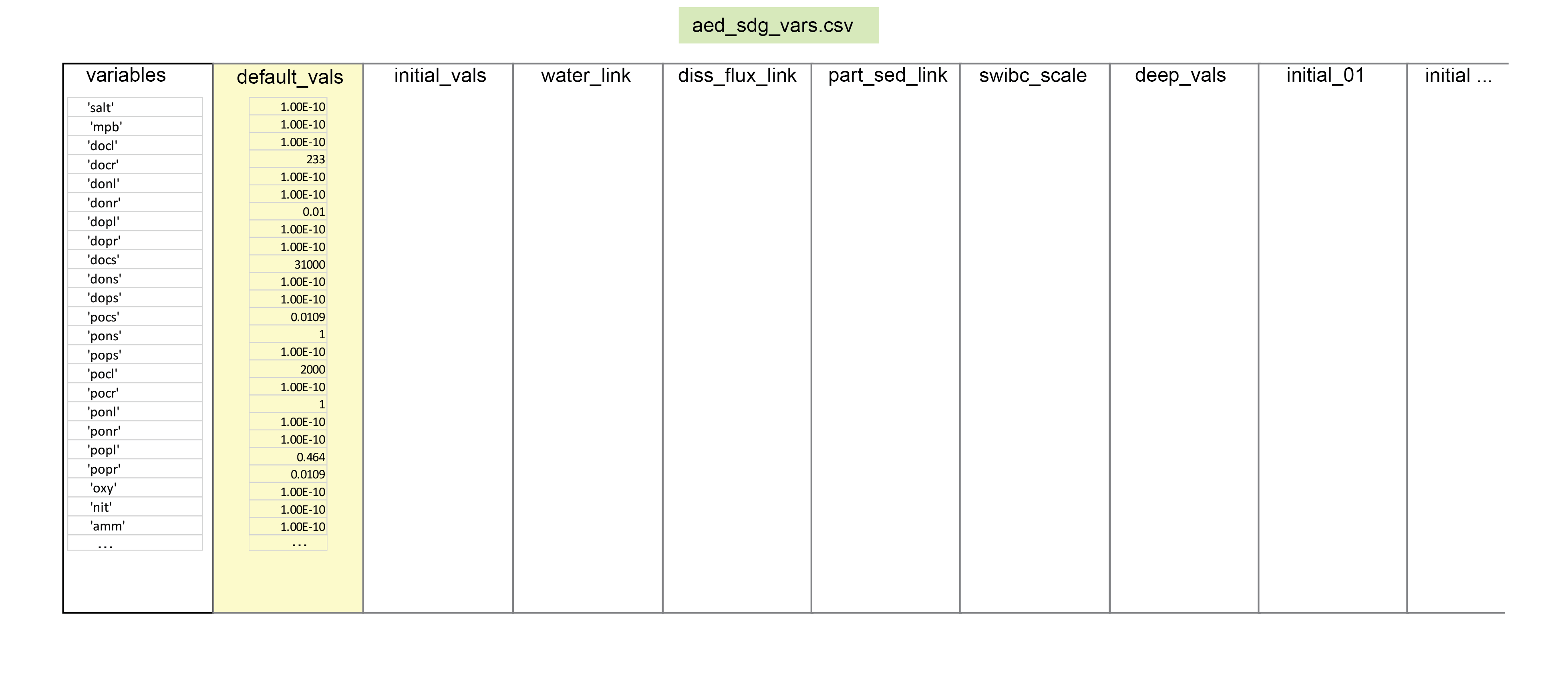
Figure 14.36: Simplified image of the aed_sdg_vars.csv input file. The variables and default_vals need to be set for each row of the csv.

Dynamic options: linked variables

There are four methods for linking variables to the water column model: - particle deposition flux using part_sed_link - solute flux using diss_flux_link - bottom water concentration using water_link - fixed linked variables

These do not need to be set for any variable, but they may be set for any variable. part_sed_link and water_link must be set for solids and solutes and cannot both be assigned to one variable. If a variable is not set to be linked, the csv contains double inverted commas (” “) and the value is set to the default_vals. To enable this option, set swibc_mode = 0.

As mentioned above, where there is any mismatch between the sediment and water column variables, the factor of part_sed_scale can be used. part_sed_scale can be found in the file aed_sdg_vars.csv. part_sed_scale is a real number between zero and one. For any sediment variables linked to the same water column flux, the part_sed_scale values should sum to 1.

If a variable is linked, it is linked for all zones.

Environmental variables have a fixed link to the water column: $Salinity$, $Temperature$ and $\tau_b$. These variables are key components of hydrodynamic models but do not undergo any rates of change in the sediment model. They are used to affect other sediment processes. As mentioned in the Environmental variables section, the $SO_4^{2-}$ concentration (mmol L^-1) is fixed at 0.9 $\times$ salinity (PSU).

Schematic of possible linked variable options at the sediment-water interface. Particle fluxes and bottom water concentraitons go from the water column to the sediment. Sediment solutes can also be set to flux to the water column.

Figure 14.37: Schematic of possible linked variable options at the sediment-water interface. Particle fluxes and bottom water concentraitons go from the water column to the sediment. Sediment solutes can also be set to flux to the water column.

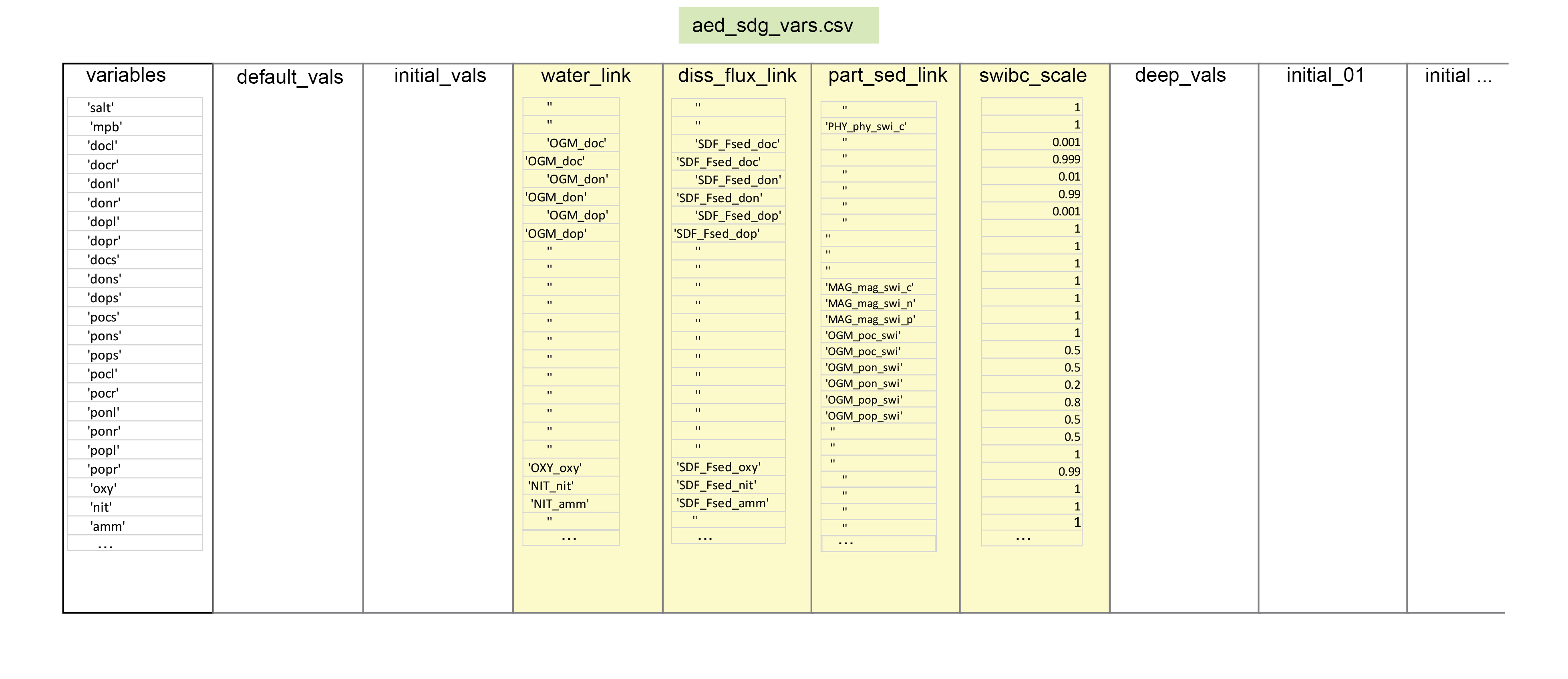
Simplified image of the `aed_sdg_vars.csv` input file. Linking variables may be set in the same row as the variable, or left blank with inverted commas.

Figure 14.38: Simplified image of the aed_sdg_vars.csv input file. Linking variables may be set in the same row as the variable, or left blank with inverted commas.

Dynamic options: swibc file

A dynamic boundary can be set for any variable and any zone using the text file swibc.dat (14.39). For a variable to be activated to take its boundary from swibc.dat, it must be included in the list swibc_filevars, which is a parameter in the &aed_sed_candi block. The specific filename and filepath are set in the parameter swibc_file in the &aed_sed_candi block. The swibc file has the following features:

timestep column: The number of the point where anything changes from the previous entry.\
time column: The time (days) at which a change occurs. Unlike a time series, each time step does not need to be listed. However, if there is a change in any one of the variables, an entry must be included in that row for all of the variables.\
forzone row: The zone for which the variable in this file applies. If a zone is not listed, then the variable in that zone will take the default_vals.\
variable columns: The value at the boundary until the next point of change.\
w00h00 columns: if any column is labelled w00h00, then a dynamic poreflux is applied to that zone.\

The benefit of using this file is that a time-changing boundary can be applied for a selection of variables and zones, while leaving other combinations of variables and zones unchanged. To enable this option, set swibc_mode = 10.

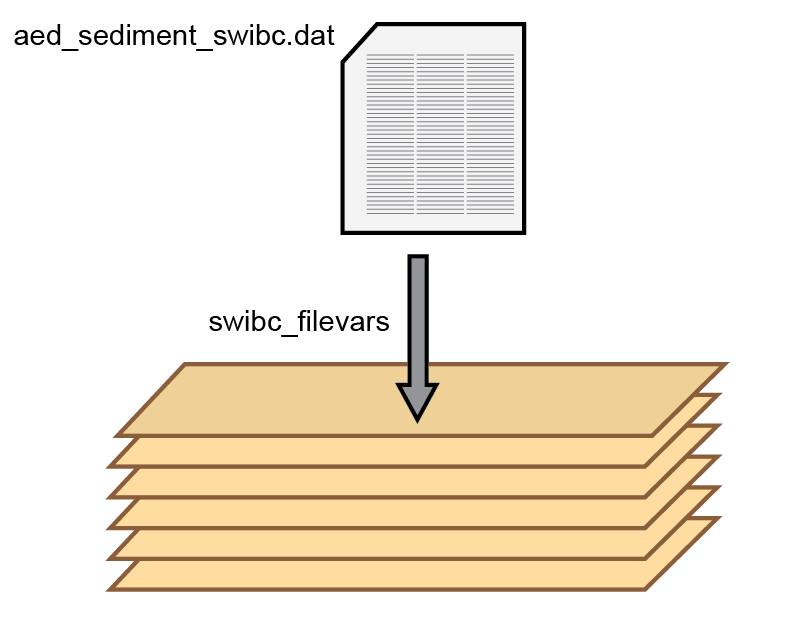
Figure 14.39: Schematic of the sediment-water interface boundary supplied by the swibc.dat text file.

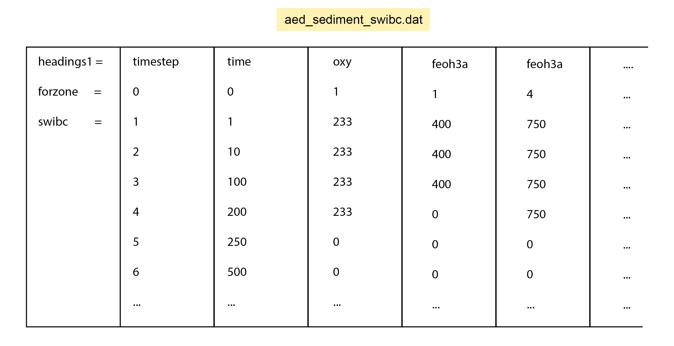
Figure 14.40: Simplified image of the swibc.dat text file.

Special organic matter flux

The sediment model has a unique boundary condition, where a large influx of organic matter occurs for a limited time (figure 14.41). This represents, for example, the operation of a fish farm, a large algal bloom or an illegal dump of organic waste into a lake. This is a convenient tool for looking at the effect of large amounts of organic matter on other chemical species, and it operates separately to the constant flux boundaries, the swibc input file, or the variables linked to the pelagic model. The flux defaults to 0.0 before the time parameter fluxon and after the time parameter fluxoff (y). The state variable switched on by this flux is $POM_{Special}$. It is not named as, for example, labile or refractory because the user can tailor its properties to the simulation. The breakdown parameter for $POM_{Special}$ is pomspecial2dic (y^-1). The parameter ibc2 must be set to 10 or 0 for this feature to operate. The magnitude of $POM_{Special}$ flux is set in the file aed_sdg_vars.csv, in the default_vals column, and the default flux before fluxon and after fluxoff times is zero. To enable this option, set swibc_mode = 2.

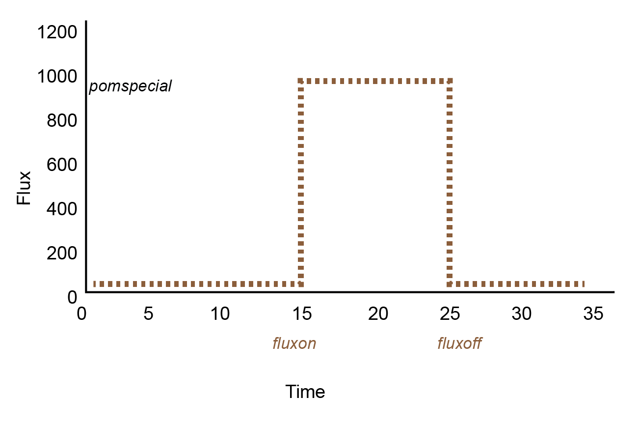
$Schematic of $POM_{Special}$ flux over time. $POM_{Special}$ flux begins at time `fluxon` and stops at time `fluxoff`. The rate of the flux is `pomspecial`.$

Figure 14.41: Schematic of $POM_{Special}$ flux over time. $POM_{Special}$ flux begins at time fluxon and stops at time fluxoff. The rate of the flux is pomspecial.

Combined organic matter flux and timestep switch

A large influx of organic matter can have the same effect for the model as processing the initial condition, and so the large flux can crash the model well after the initial spinup (figure 14.42). Therefore, further substep parameters are available for slowing the model while it processes the organic matter. The parameter substep_2 is used as the substep after fluxon. The parameter substep_3 is used as an intermediate substep after fluxoff, until the time justwaitabit, to allow the final effects of the organic matter influx to be processed, but allowing the possibility of running faster if not at the speed of substep_1. Further substep options are explained in the timing switches section.

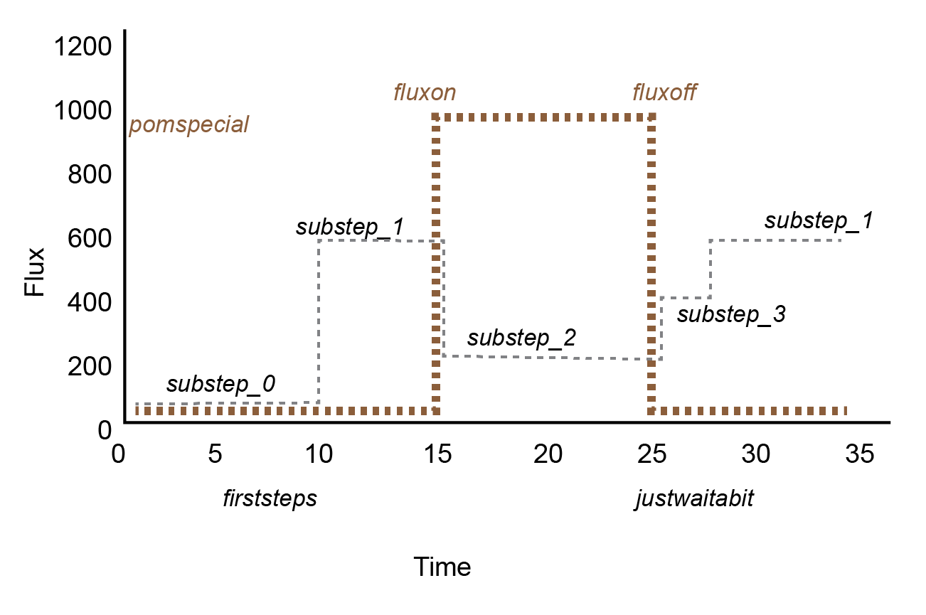
$Schematic of $POM_{Special}$ flux and timestep changes over time. Options are available to optimise a short run total time with a slow substep centred around organic matter influx.$

Figure 14.42: Schematic of $POM_{Special}$ flux and timestep changes over time. Options are available to optimise a short run total time with a slow substep centred around organic matter influx.

Bottom boundary

Static option: deep_vals

A boundary can be supplied beneath the deepest cell using deep_vals (14.43). The value is taken from deep_vals, which is in the input file aed_sdg_vars.csv (14.44). (deep_vals is the lower boundary equivalent of the sediment-water interface default_vals.) In most instances a bottom boundary would not be supplied, however, if there were a simulation with, for example, groundwater infiltration, then this option is used. If the value in deep_vals is negative, no boundary is applied, and so the file has a default -999 for all variables. To enable this option, set deepbc_mode = 1.

Figure 14.43: Bottom boundary inputs that are constant in time are set with deep_vals.

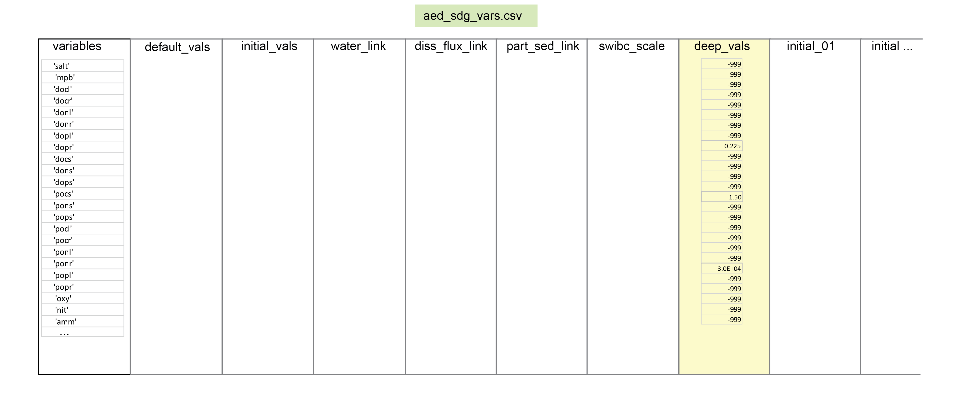
Simplified image of the `aed_sdg_vars.csv` input file. deep_vals are set if a value is present, greater than zero, corresponding to a variable.

Figure 14.44: Simplified image of the aed_sdg_vars.csv input file. deep_vals are set if a value is present, greater than zero, corresponding to a variable.

Dynamic option: deep_bc file

A dynamic boundary can be set for any variable and any zone using the text file deepbc.dat (14.45). For a variable to be activated to take its boundary from deepbc.dat, it must be included in the list deebc_filevars, which is a parameter in the &aed_sed_candi block. The specific filename and filepath are set in the parameter deepbc_file in the &aed_sed_candi block. The deepbc file is the bottom boundary equivalent of the swibc file. It has the following features:

timestep column: The number of the point where anything changes from the previous entry.\
time column: The time (days) at which a change occurs. Unlike a time series, each time step does not need to be listed. However, if there is a change in any one of the variables, an entry must be included in that row for all of the variables.\
forzone row: The zone for which the variable in this file applies. If a zone is not listed, then the variable in that zone will take the default_vals.\
variable columns: The value at the boundary until the next point of change.\
pf columns: if any column is labelled pf, then a dynamic poreflux is applied to that zone.

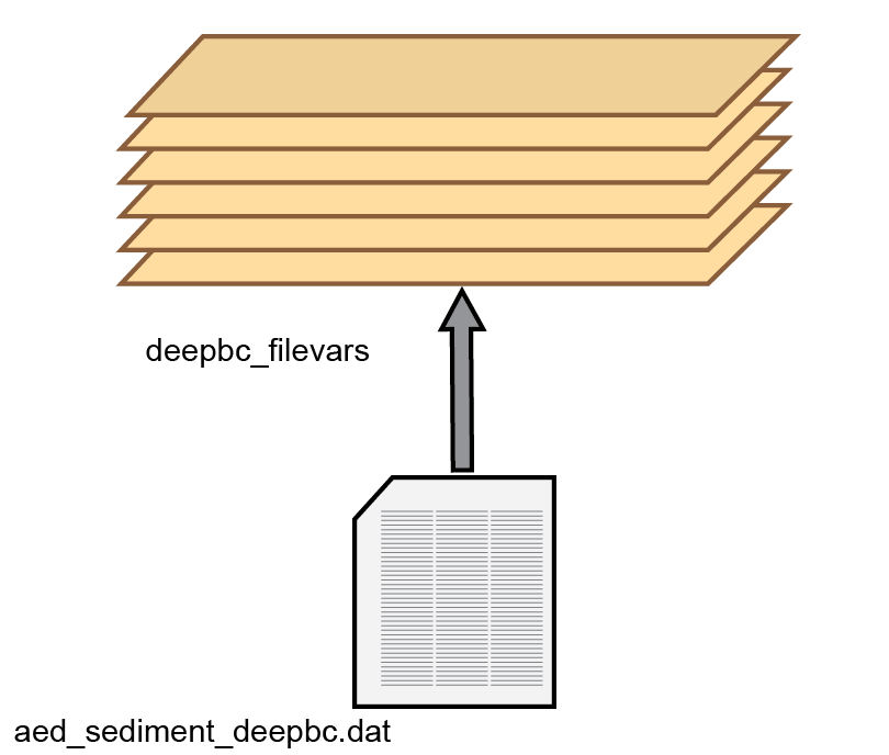
Figure 14.45: Schematic of the bottom boundary supplied by the deepbc.dat text file.

14.5 Output & Post-processing

CANDI-AED has a range of output files and output file options.

14.5.1 Concentration of state variables: ‘.sed’ files

The model writes output files for each state variable (chemical species, $IAP$s, $pH$, $pe$ and $ubalchg$) as text files, with a ‘.sed’ extension. The files are written to the results directory, under the candi_aed subdirectory, and then in a separate subdirectory for each zone (with five significant figures), for example .../results/candi_aed/00001/oxy.sed. The ‘.sed’ file has three rows of headers, then a row that lists the depths (cm). The first column is the sequence of output times (years). The other text entries are a matrix of the concentration values at each depth and each time (mmol L^-1) (figure 14.46). These can be read in using a data processing program such as R, Matlab or Excel for analysis and plotting 14.47.

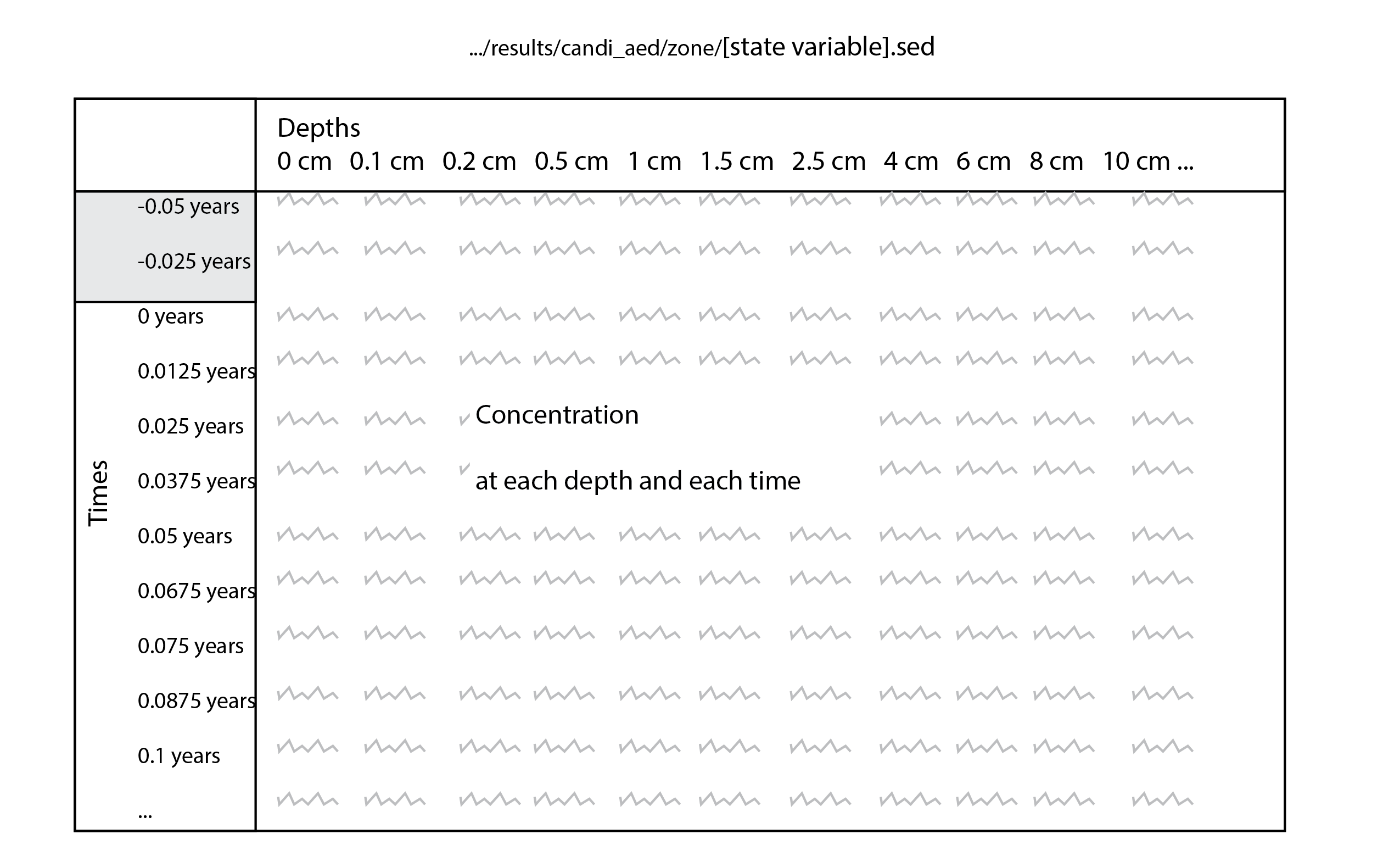
Figure 14.46: Simplified version of the .sed output file.

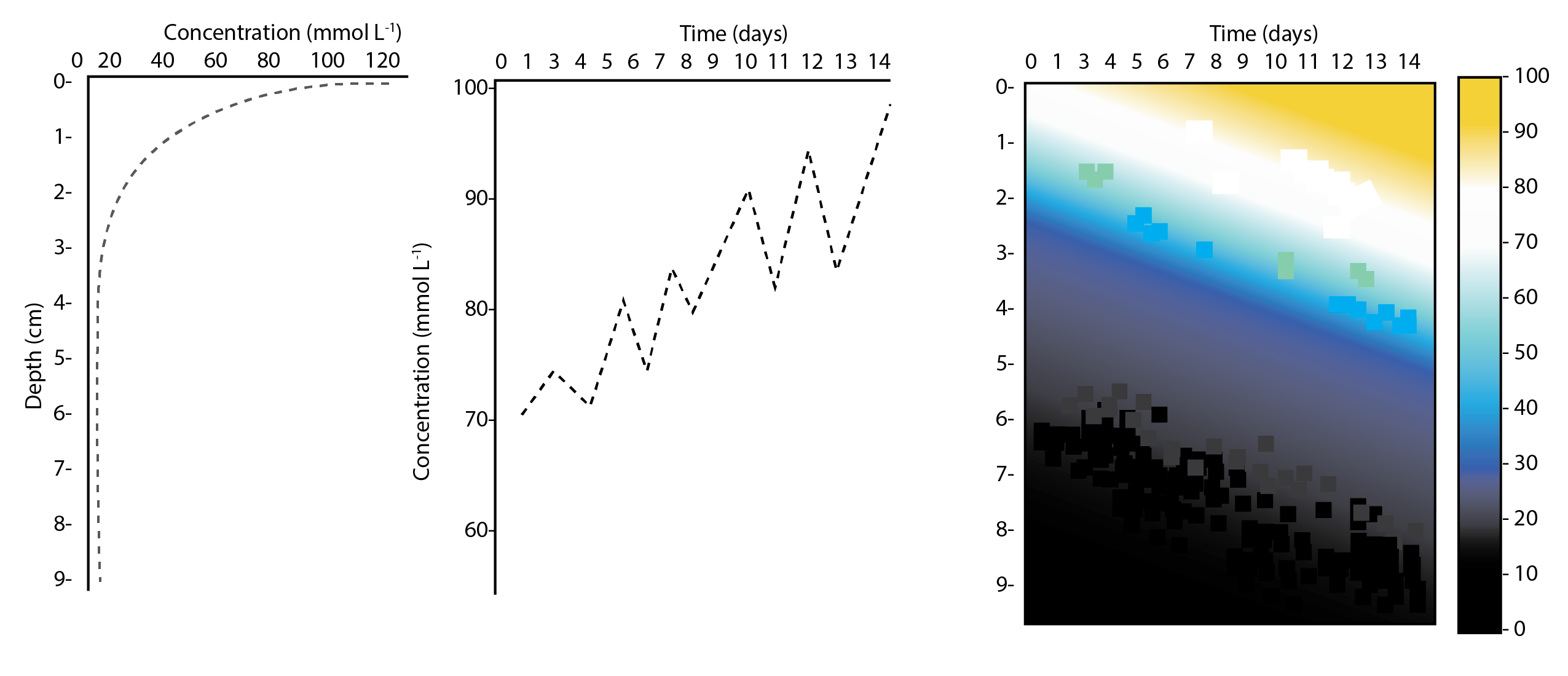
Examples of the figures that can be plotted with the .sed file. Left: concentration-depth at one time step; centre: concentration-time at one depth; right: concentration-depth-time

Figure 14.47: Examples of the figures that can be plotted with the .sed file. Left: concentration-depth at one time step; centre: concentration-time at one depth; right: concentration-depth-time

14.5.2 Flux of state variables: ‘swi_fluxes.sed’

The model writes output files for sediment-water interface fluxes, named swi_fluxes.sed. As with the concentration ‘.sed’ files, the ‘swi_fluxes’ files are written to the results directory, under the candi_aed subdirectory, and then in a separate subdirectory for each zone (with five significant figures), for example .../results/candi_aed/00001/swi_fluxes.sed. The file has one row of the names of all state variables, and the second row for whether the variables are solids or solutes. The first column is the sequence of output times (years). Only the post-spinup times (positive time) are written to the file, as there are no fluxes during spinup. The other text entries are the flux values (mmol ^-2 y^-1), where a positive value is a flux into the sediment, and a negative value is a flux to the bottom water (figure 14.48). As with the ‘.sed’ files, these files can be processed and plotted (14.49).

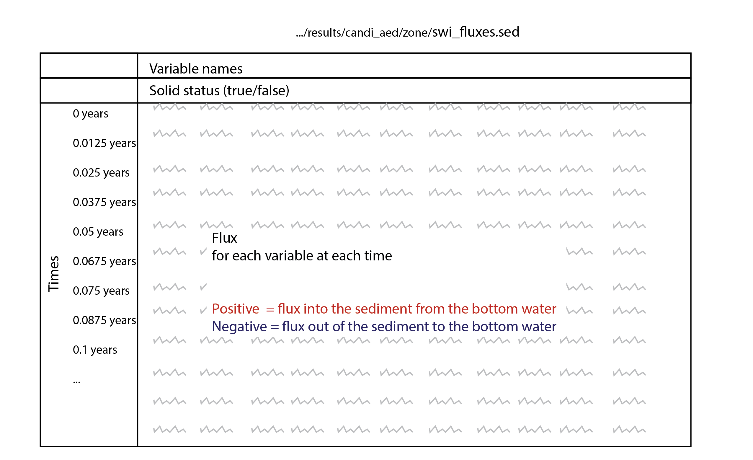
Figure 14.48: Simplified version of the swi_fluxes.sed file.

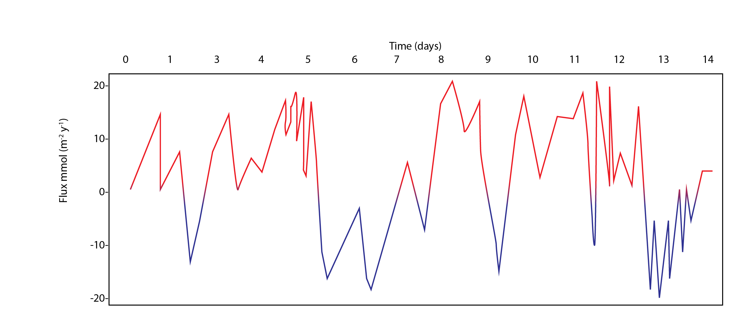
Figure 14.49: Example of a figure that can be plotted from fluxes.sed

14.5.3 Other variables: ‘/Extras/ .sed’

Any variable listed in the &aed_sed_candi block parameter morevariables can be written if to a file if desired. Extra ‘.sed’ files can be written to a subdirectory of the zone directory, for example .../results/candi_aed/00001/Extras/RO2.sed. The file has the same format as the other ‘.sed’ files, however, it does not record values during the spinup period (figure 14.50). The unit of the variable is dependent on what is used in the model code and there is no unit conversion before the file is written.

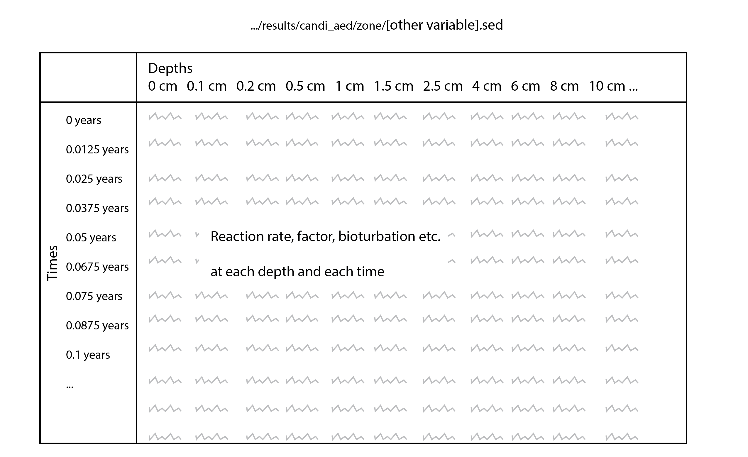
Figure 14.50: Simplified version of the extra .sed file.

14.5.4 Depth profile settings: ‘Depths.sed’

The model writes a text file that reports the initial depth profile settings, with one entry per layer (maxnpts). One file is written for each sediment zone and it is not updated throughout the simulation, for example .../results/candi_aed/00001/Depths.sed. The file can be useful in post-processing, including performing unit conversions. The outputs include

Depths: The depths of the grid layers from the sediment-water interface (cm)
Porosity: The volume of water per volume of space, between 0 and 1
Irrigation: The initial irrigation
Bioturbation: The initial bioturbation
Layer_size_cm: The sizes of the layers (cm)
Porewater_m3_per_m2: The volume of porewater in each layer (m³ m^-2)
Solids_m3_per_m2: The volume of sediment solids (m³ m^-2)

14.5.5 Mass balance calculation

The function Mass within the CANDI-AED code calculates the mass balance of some species.

Firstly it calculates FOM_in, which is the influx of

14.6 Case Studies & Examples

Several case studies are outlined below.

Numerical mass balance and flux confirmation

Mass check approach

It is important to check that a simulation is conserving mass in the upper layers of the sediment because with the wrong settings, numerical errors can lead to the wrong calculation of sediment mass. One method for checking for errors involved a non-reactive solid and a non-reactive solute being introduced at the sediment-water interface (SWI) as ‘tracers’. As they enter at the SWI, the tracers’ fluxes and concentrations were converted to mass units, per 1 m$^2$. The concentrations in the sediment were similarly summmed per 1 m$^2$, across all depths.

Mass check methods

General settings

The sediment model was run with no variables except one solid (organic matter) and one solute (N2) ‘tracer’, the reaction rates of which were set to zero. The tracers were applied as fluxes and concentrations at the sediment-water interface boundary. The simulation had

no influx for 0.5 years to check that the model had equilibrated, then
the boundary flux or concentration was applied for 1 year, then
the boundary was switched off and the simulation run for a further year.

The mass of influxing matter was calculated. Key parameters were changed one by one and a range of simulations was run, in order to check for possible mass balance errors.

Settings investigated for errors

Key parameters that were varied included

either a fixed grid or exponentially increasing layers
grid spacing and time steps
solid sedimentation rates (ω00)
porosity (ρ0 and ρ00)
bioturbation depths and functions

SWI specific settings

‘aed.nml’ settings:

‘swibc_mode’ = 10 (integer switch). The boundary to the file listed in ‘swibc_file’.
‘swibc_file’ = ‘swibc.dat’ (filename). The sediment-water interface boundary condition (SWIBC) file in the aed_sdg folder.
‘swibc_filevars’ = ‘pomspecial’, ‘n2’ (variable names). The variables taken from the swibc file.

‘aed_candi_params.csv’ settings:

‘OMModel’ = 1 (integer switch). The simplest organic matter reaction model.
‘pomspecial2dic’ = 0 (y$^{-1}$). The ‘pomspecial’ that fluxes in is unreactive.

The ‘pomspecial’ flux was 1.0E-08 (mmol m$^{-2}$ y$^{-1}$) and the ‘n2’ concentration was 1.0E-08 (mmol m$^{-3}$) for most of the simulation. The model converted the concentration from mmol m$^{-3}$ to mmol L$^{-1}$.

At time 183 days (or 0.5 years) the flux and concentration increased to 1.0E+02 (mmol m$^{-2}$ y$^{-1}$) and 1.0E+05 (mmol m$^{-3}$). At 548 days (or 1.5 years) the flux and concentration returned to the very low number.

Grid settings

‘aed_candi_params.csv’ settings:

‘job’ = 0 (integer switch). An evenly-spaced grid.
‘p0’ = 0.5 (fraction between 0 and 1). The porosity at the sediment-water interface.
‘p00’ = 0.5 (fraction between 0 and 1). The porosity at depth. These porosities were set to be the same, which gave the most reliable results.
‘imix’ = 2 (integer switch). The bioturbation set to have exponential decay rather than the sharper cutoffs with ‘imix’ = 1.
‘maxnpts’ = 41 (layers). With ‘job’ = 0 this must a multiple of the depth (cm) + 1 layer (for the zeroth layer), for example, 81, 201 or 401.
‘xl’ = 20 (cm). This depth was adequate for this simulation.
‘xirrig’ = 3 (cm). The depth of irrigation.
‘xs’ = 5. The shape of the decay curve for bioturbation.

Mass calculation method

This section outlines the method for calculating the mass. There are many steps in the path to convert all of the quantities, starting with input parameters, calculations in the model, outputs from the model, and post-processing in R. An error in the assumptions behind or calculation of any of these steps would give a false idea of whether mass was being maintained.

Parameter inputs

Porosity is assigned in aed_candi_params.csv, using the parameters ‘p0’ and ‘p00’, setting porosity at the highest and lowest layers.

Internal calculations

‘aed_secandi’ calculates the variable ‘poros’ as an exponential decay from ‘p0’ to ‘p00’.

‘poros’ is used to calculate ‘ps’ (1 - poros). ‘ps’ and ‘poros’ are used to calculate the ‘psp’ and ‘pps’ as ‘ps’/‘poros’ and ‘poros’/‘ps’. These are ratios of porosity that are used to convert solid and solute units elsewhere in candi. For example, as ‘Fe(OH)3A’ (solid) reduces to ‘Fe$^{2+}$’ (solute) it is multiplied by ‘psp’ to convert the units from mmol L $^{-1}$ solids to mmol L $^{-1}$ (porewater).

Two other variables are calculated within ‘aed_sedcandi’, using ‘dh’, which is the distance between sediment layers (cm). The porewater volume variable, ‘porevol’, is calculated as ‘dh’ / 100 $\times$ ‘poros’. The solid volume variable, ‘solvol’, is calculated as ‘dh’ / 100 $\times$ 1 - ‘poros’. These are then expressed as m$^3$ of porewater or solids per 1 m$^2$.

Model outputs

The model produces solid variables in units of mmol / L $^{-1}$ (solids) and solute variables in units of mmol L $^{-1}$ (porewater). These are written as concentrations over time, across all depths.

The model also produces a time series of SWI fluxes. These are in units of mmol m$^{-2}$ y^{-1}, where the area component is total area of space, rather than the area of solids or porewater.

It also outputs ‘porevol’ and ‘solvol’, with entries per depth, but without time, since they do not change over time.

R post-processing

In processing the SWI fluxes file, the fluxes are converted via the following steps:

raw output is in mmol m$^-2$ y$^-1$ / 1000
mol m$^-2$ y$^-1$ $\times$ molecular mass
cumulative [t] g m$^-2$ = cumulative[t-1] g m$^-2$ + g m$^-2$ y$^-1$ [t] $\times$ (time[t] - time[t-1])

This gives a time series of influxed mass per 1 m$^-2$.

The mass in the sediment is converted via the following steps:

raw output is in mmol L$^-1$
if the variable is a solid, the concentration is multiplied by solvol and 1000. mmol L^-1 $\times$ m$^3$ of solids per 1 m $^2$ = mmol solids per 1 m$^2$
- if the variable is a solute, the concentration is multiplied by porevol and 1000. mmol L^-1 $\times$ m$^3$ of porewater per 1 m$^2$ = mmol porewater per 1 m$^2$
mmol m$^{-2}$ / 1000 = mol m$^{-2}$
mol m$^{-2}$ $\times$ molecular mass = g m$^{-2}$
this matrix of mass m$^{-2}$ is then summed over all depths at each time. This gives a similar time series of mass per 1 m$^{-2}$.
for plotting, this is then carved into three sections, 0 cm to 1 cm, 1 cm to 2 cm, and 2 cm to the bottom. This does not affect the total mass.

Mass check results

Mass check base case

Simulations were run with a non-reactive solute and solid to check that the total influxing mass was equal to the mass across all layers of the sediment. Parameters and settings were changed until the masses were the same and the model could be used with confidence. The bottom left panel in each figure shows the sediment mass as the shaded area, and the influxed mass as the red line. An equal grid spacing was used to minimise possible large concentration differences between layers. The model was run quickly with 5-daily time steps, which had no effect on model error. The most important setting was that the initial bioturbation profile was set to the exponential decay option rather than the two-layer option (imix = 2 rather than 1, see chapter 14.3.2.6 for details) because it was found that the sharp cutoff of the two-layer option was prone to small numerical errors, when the concentration differences between layers were large. With the exponential decay setting, bioturbation decreased from its maximum value at the sediment water interface to 10 cm deep.

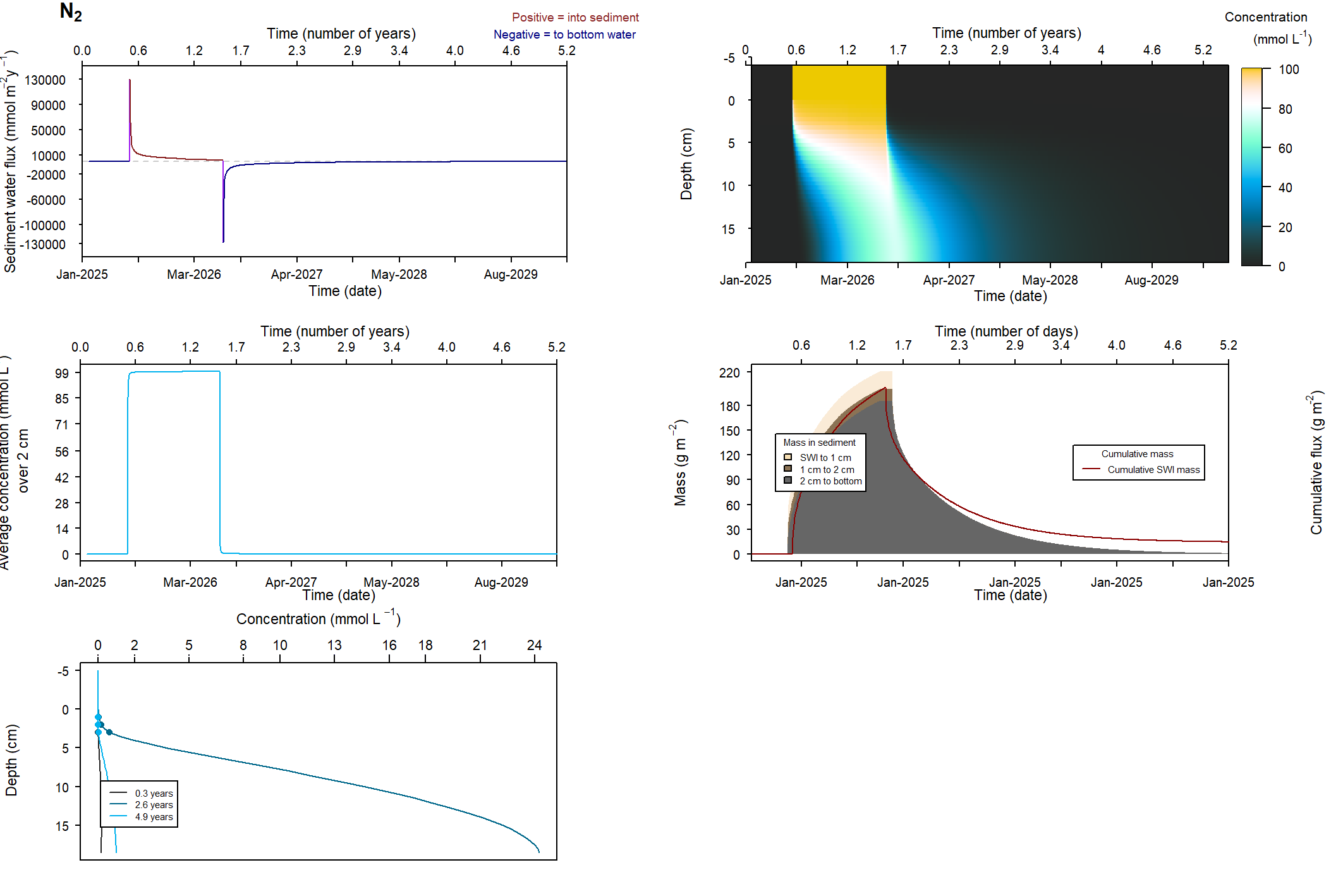
Results of a simulation for $N_2$ as a tracer. Reaction rates were turned to zero and so concentration and mass changes are the result of transport only. After 6 months of spin-up, both species were introduced at the sediment-water interface for one year. The bottom left figure showed that the total sediment mass and influxing mass were the same.

Figure 14.51: Results of a simulation for $N_2$ as a tracer. Reaction rates were turned to zero and so concentration and mass changes are the result of transport only. After 6 months of spin-up, both species were introduced at the sediment-water interface for one year. The bottom left figure showed that the total sediment mass and influxing mass were the same.

Results of a simulation for organic matter. Reaction rates were turned to zero and so concentration and mass changes are the result of transport only. After 6 months of spin-up, both species were introduced at the sediment-water interface for one year. The bottom left figure showed that the total sediment mass and influxing mass were the same.

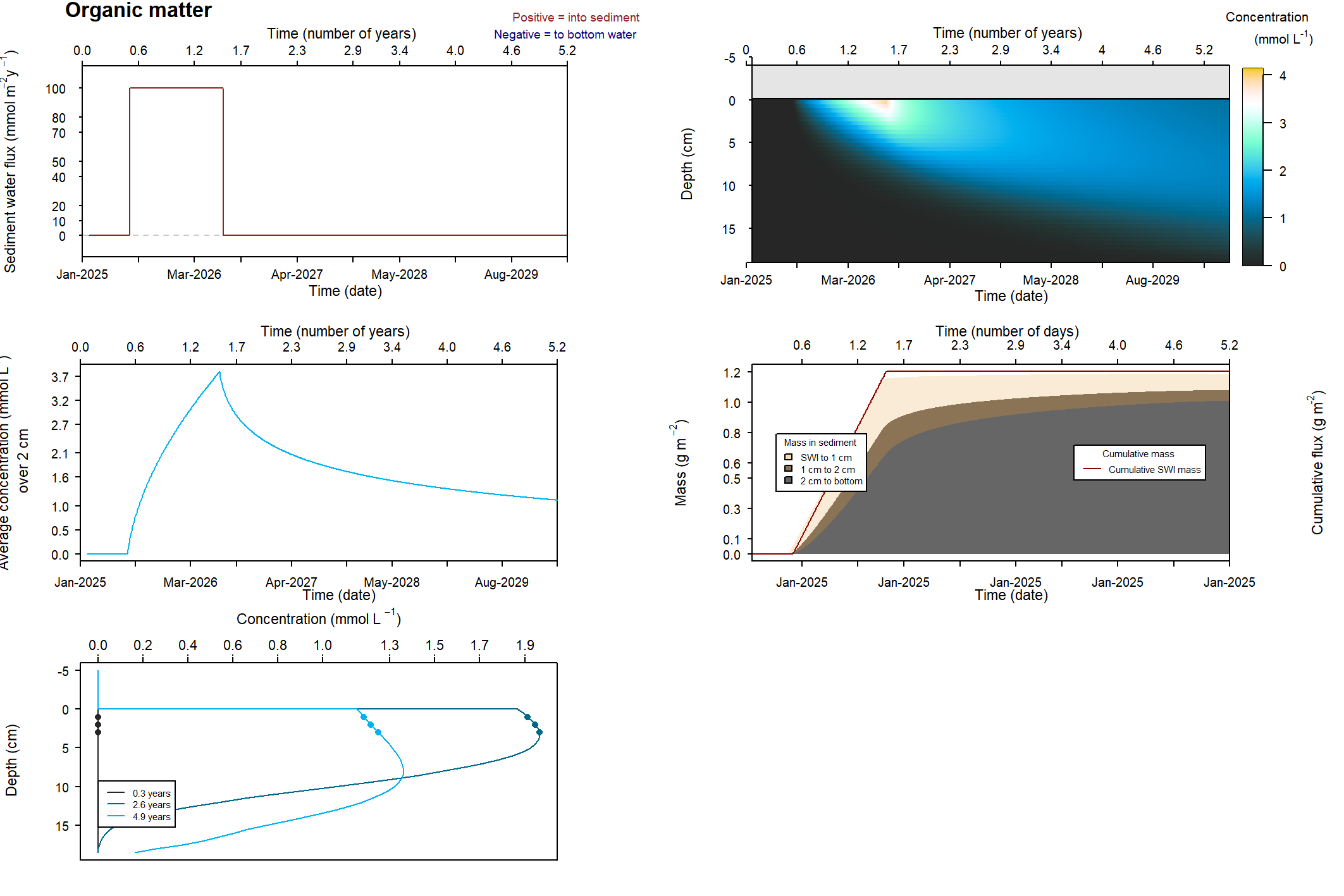
Figure 14.52: Results of a simulation for organic matter. Reaction rates were turned to zero and so concentration and mass changes are the result of transport only. After 6 months of spin-up, both species were introduced at the sediment-water interface for one year. The bottom left figure showed that the total sediment mass and influxing mass were the same.

Deliberate errors - high porosity

Parameters ‘p0’ and ‘p00’ were set to 0.75. This resulted in a good solid balance but a higher sediment mass than influxed mass for solutes.

With high porosity, the solid mass reconciled well but the solute mass was higher in the sediment than from the influx. The maximum mass of solute was around 350 g m$^-2$.

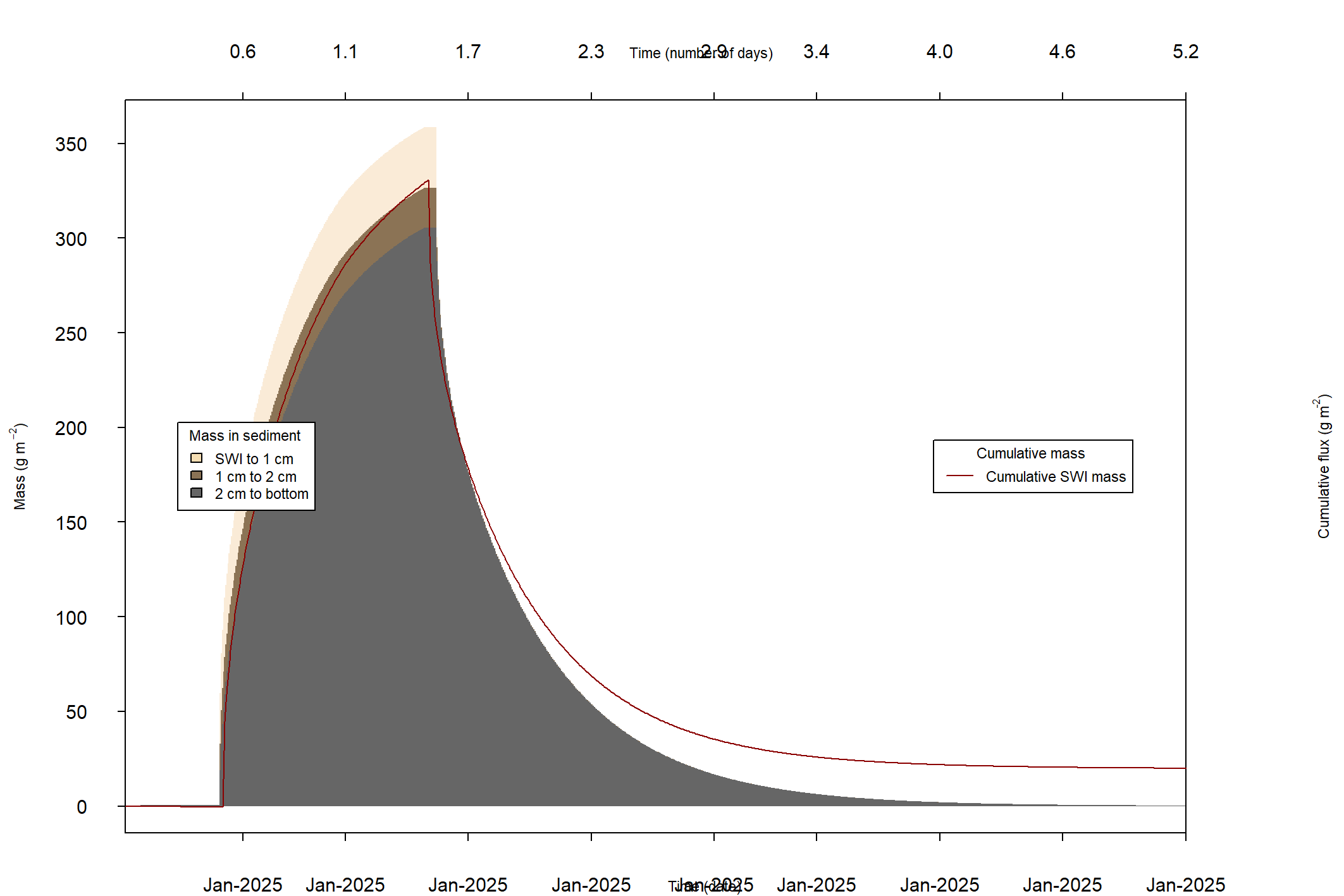
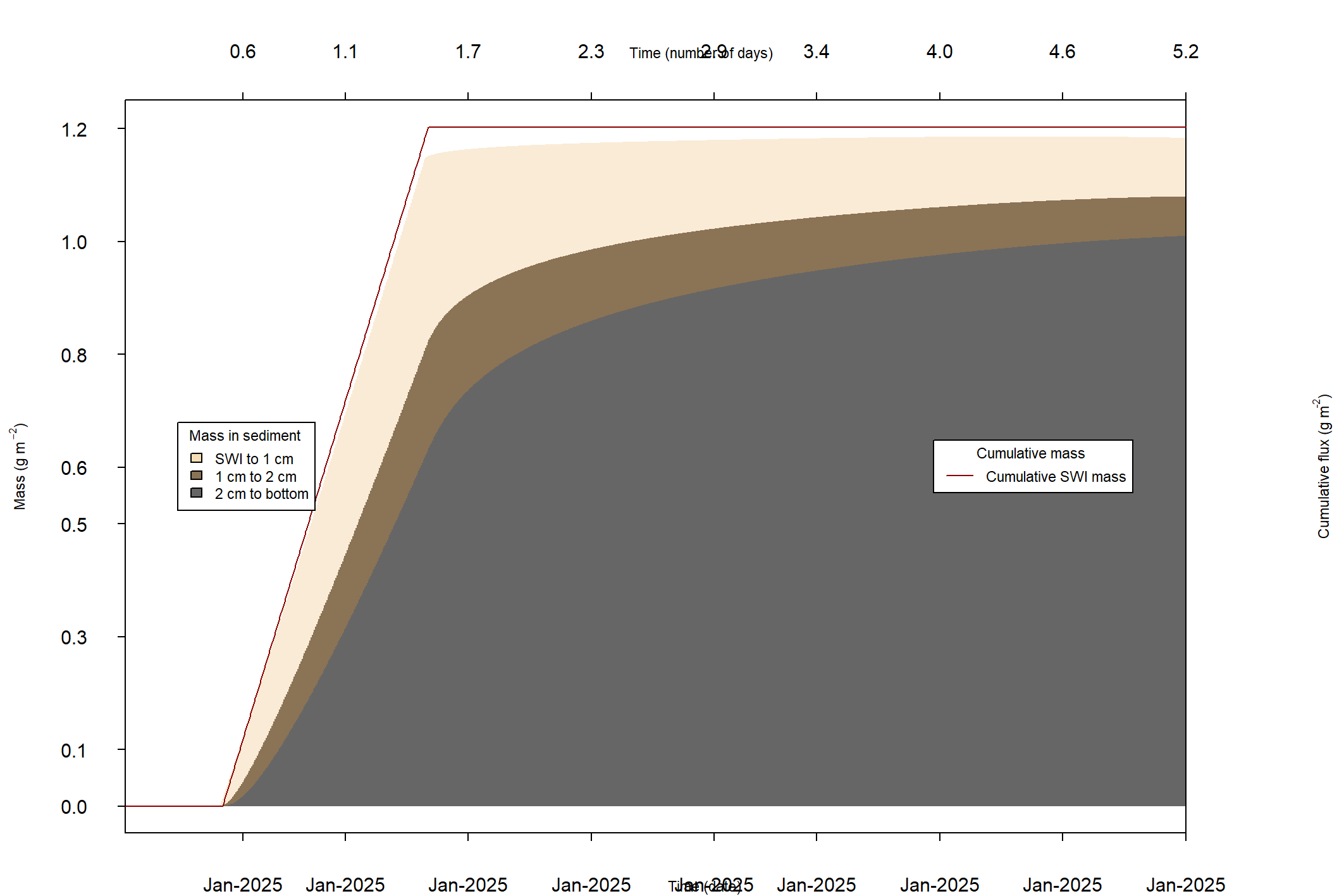
Deliberate errors - low porosity

Parameters ‘p0’ and ‘p00’ were set to 0.75. This resulted in a good solid balance but a higher sediment mass than influxed mass for solutes.

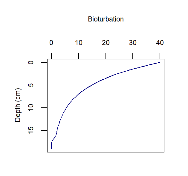
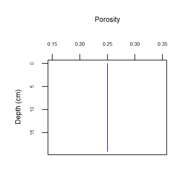
With low porosity, as with high porosity, the solid mass reconciled well but the solute mass was higher in the sediment than from the influx. The absolute mass of solid was the same with high or low porosity, however, the maximum mass of solute was approximately 100 g m$^2$.

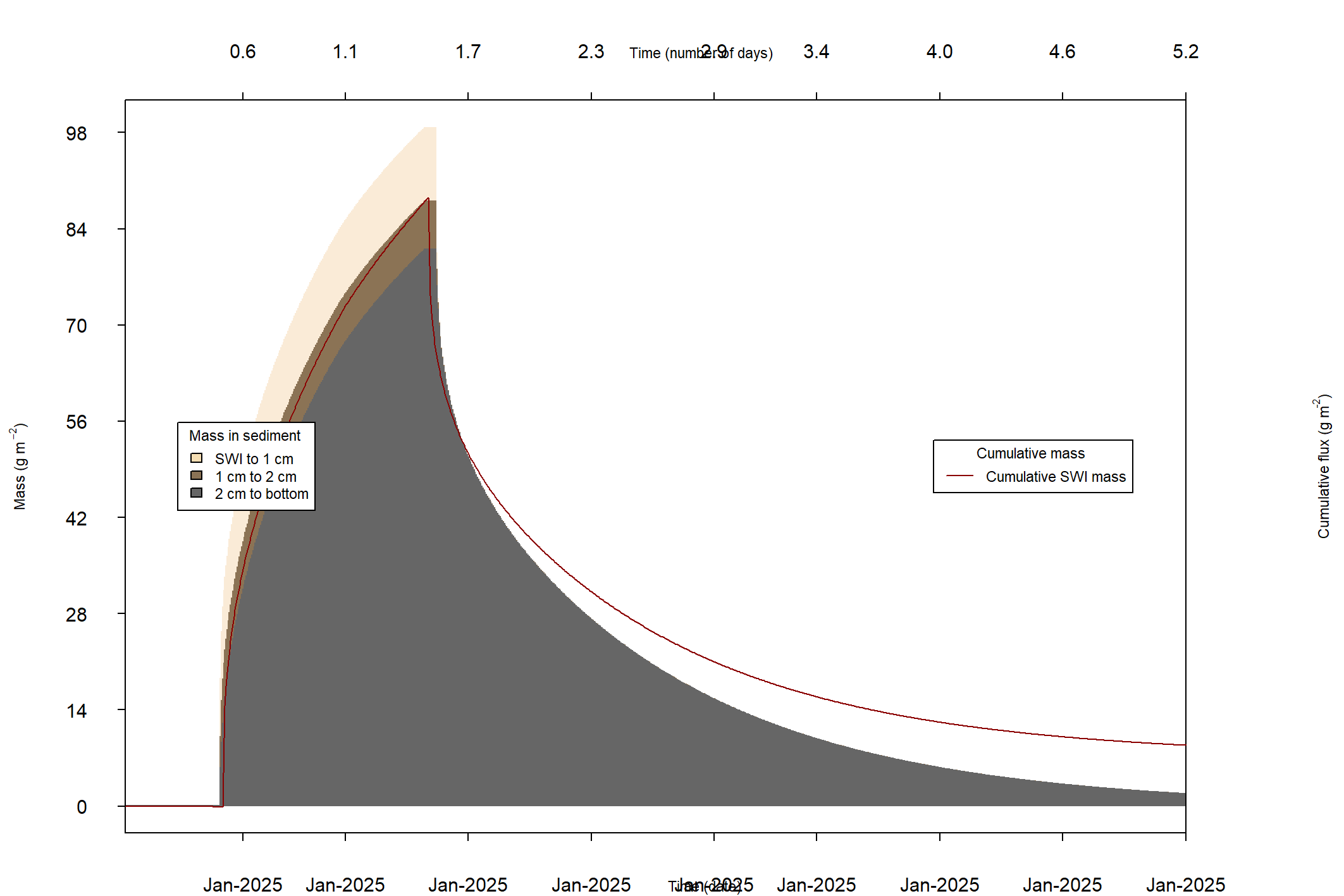
Deliberate errors - porosity gradient

Parameters ‘p0’ was set to 0.9 and ‘p00’ to 0.5.

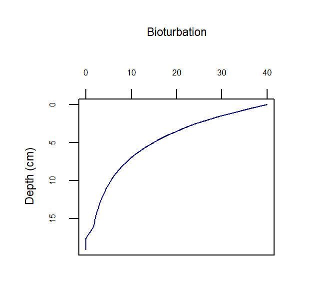
This created the clearest error. Reported sediment mass was much lower than influxed mass.

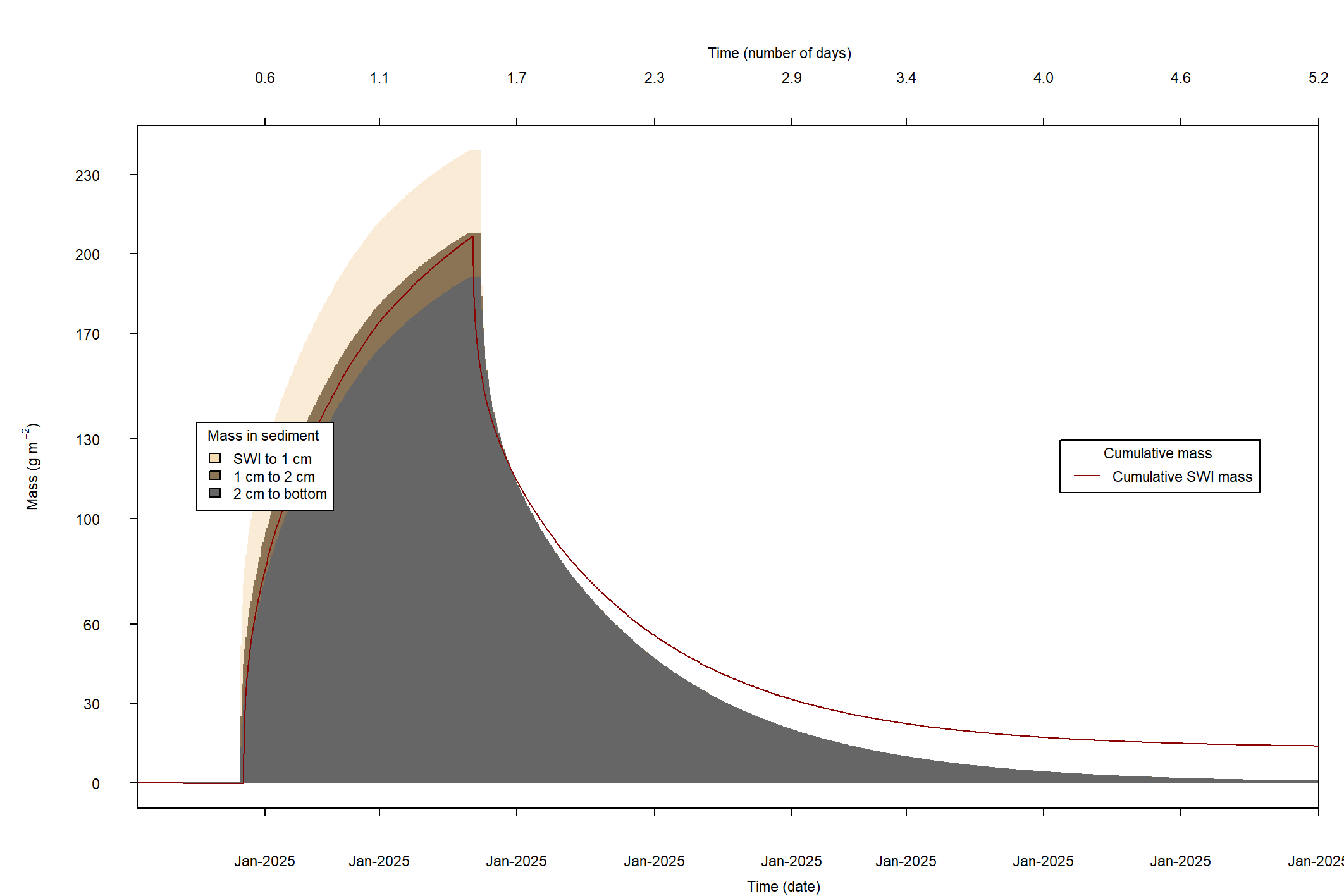
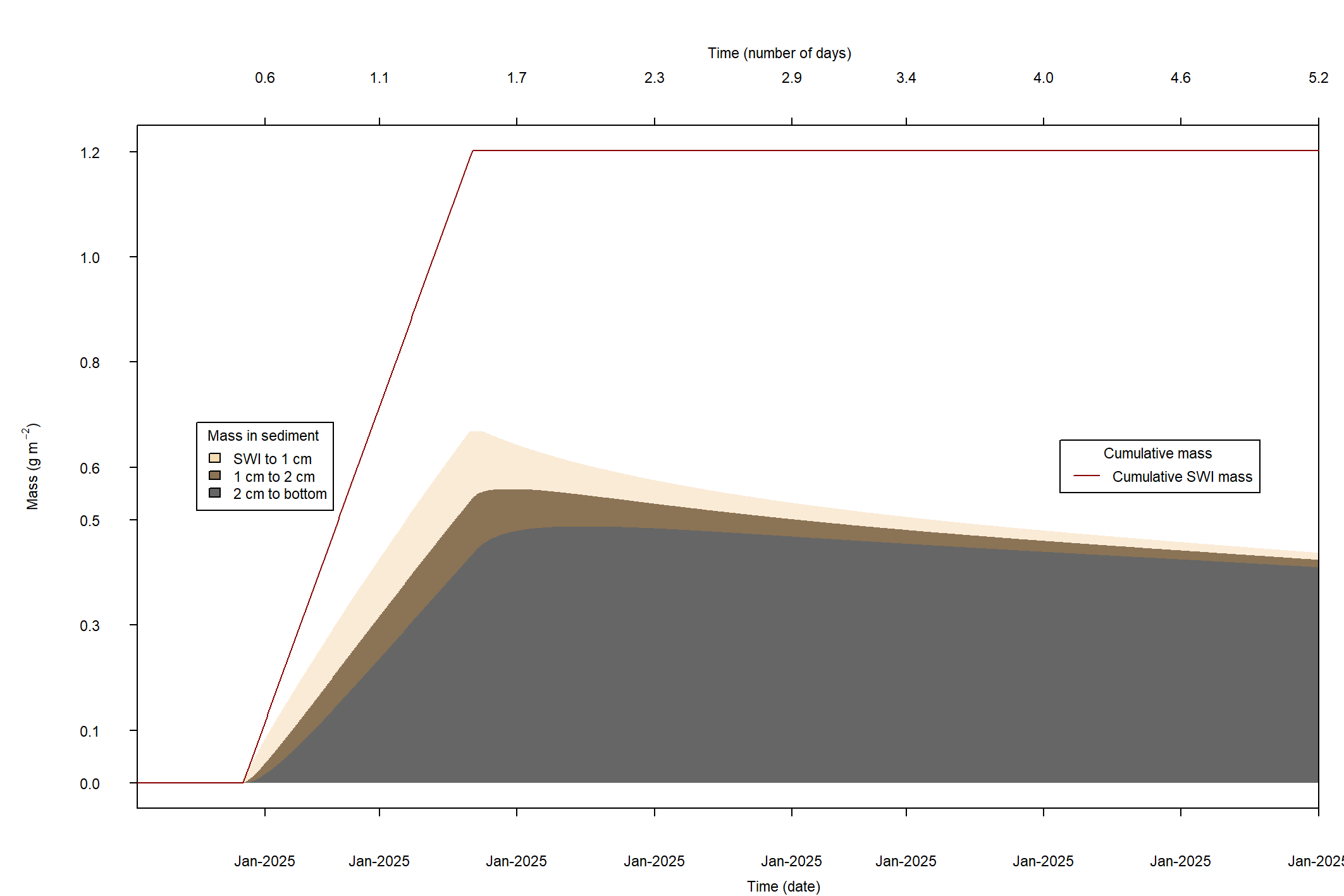
Bioturbation settings

In this setup, bioturbation does not cause a problem with mass. However, future simulations with different bioturbation settings should be checked for mass conservation. One of the primary risks is having a sharp cutoff for bioturation at two depths.

The bioturbation intensity, ‘DB0’, might also affect the mass conservation.

14.6.1 Case study: Model benchmark example

14.6.1.1 Model setup

Base simulation

The model CANDI-AED was tested against the published modelling results of Van Cappellen and Wang (1996) in order to confirm that the model worked as expected, and also to demonstrate the flexibility of the model system. For this simulation, all boundary fluxes, bottom water concentrations, and rate constants were set to the same values as those in Van Cappellen and Wang (1996). The organic matter redox approach was set to Approach 2, by setting OMApproach = 2. The organic matter oxidation model was parameterized with no organic matter influx and with an oxidation rate that changes with depth (OMModel = 1, VCW = TRUE). The surface oxidation rate and depth attenuation were the same as Van Cappellen and Wang (1996). The irrigation coefficient was also set to be the same as in Van Cappellen and Wang (1996), using irrigswitch = 2. The mineral precipitation reactions were implemented only for MnCO3, FeCO3 and FeS, as per the equations in Van Cappellen and Wang (1996), rather than the larger set of precipitation reactions (rxn_mode = 4). Additionally, the ageing reactions of iron and manganese minerals were disabled. Ammonium adsorption was included and was the same as in Van Cappellen and Wang (1996), however, iron and manganese adsorption has not yet been included. An equivalent evenly spaced grid was used (job = 1), with 400 layers (mxnpts) to a depth of 20 cm (xl).

Parameter variation

The model was run with random variation in its parameter values, to assess the sensitivity of the outputs to the parameter values. The base simulation above was run again with variations of the uncertain parameters listed in Table 6 of Van Cappellen and Wang (1996). Rather than using the ranges that Van Cappellen and Wang used, the range was set using their chosen parameter value as the median. 100 simulations were run using a Matlab script, with individual parameter values automatically generated using a Monte Carlo-based method. The results of each simulation were then collated and the total results were assessed for distribution about the median value.

Table 14.24: Parameters varied in the uncertainty analysis, within the ranges chosen by Van Cappellen and Wang (1996).
Parameter	Description	Range	Unit
DB₀	Biodiffusion constant	4 to 36	cm² y^-1
x_b	Depth of biodiffusion decrease	20 to 30	cm
α₀	Bioirrigation coefficient	100 to 300	y^-1
x_irrig	Bioirrigation coefficient	0.02 to 0.54	cm
y_Lab	N:C ratio	9.6 to 32	N atoms:106 C atoms
z_Lab	P:C ratio	0.7 to 1.55	P atoms:106 C atoms
K_TEAO2	Aerobic oxidation limitation concentration	1×10^-2 to 3×10^-2	mmol L^-1
_KTEANO3	Denitrification limitation concentration	4×10^-3 to 6×10^-2	mmol L^-1
k_NH4ads	NH₄⁺ adsorption coefficient	1.1 to 1.7
k_FeOx	Kinetic rate constant for aerobic oxidation of Fe²⁺	5×10² to 5×10⁴	mmol L^-1 y^-1
k_Siddis	Siderite dissolution constant	2.5×10^-5 to 2.5×10^-3	y^-1

14.6.1.2 Results

Concentrations

The $O_2$ concentration profile matched the Van Cappellen and Wang simulation very closely, apart from the concentration at the deepest point, which was slightly higher than the field data (Figure 14.53 (a)). The results for $O_2$ were very consistent about the median value. The slightly higher concentration of oxygen at the deepest point in this simulation may have carried through to inhibit denitrification, causing the concentration of $NO_3^-$ to be higher than in the Van Cappellen and Wang simulation (Figure 14.53 (a)). $NO_3^-$ was similarly consistent about the median. The $NH_4^+$ field data points were lower than the median of these simulations but within the range of these simulations (Figure 14.53 (c)). $pH$ was between 7 and 8, and both $NH_4^+$ and $pH$ had increasing ranges with depth (Figure 14.53 (d)).

The $MnO_2$ and $Fe(OH)_{3A}$ concentrations matched the data points closely, however, the $Mn^{2+}$ and $Fe^{2+}$ concentrations in this simulation peaked at a higher concentration around 2 cm (Figure 14.53 (e) to (h)). It was suspected that this might have resulted from poor resolution of the grid, however, this simulation had the same number and size of layers as Van Cappellen and Wang. Below 5 cm deep the simulation had a lower concentration than the field data, but the deepest 5 field data points for $Fe^{2+}$ were within the ranges of the simulations.

$H_2S$ had the greatest variation relative to its concentration, which increased with depth (Figure 14.53 (i)). $FeS$ concentration had a consistently concave shape whereas the field data appeared to be concave around 3 cm deep, and the relatively high concentration of $FeS$ at 5 mmol L^-1 in the oxic zone was not within the range of these simulations (Figure 14.53 (j)). $FeS$ could be simulated close to the field data, but only by fixing the bottom boundary at 45 mmol L^-1 and not because of its precipitation from $Fe^{2+}$ and $H_2S$.

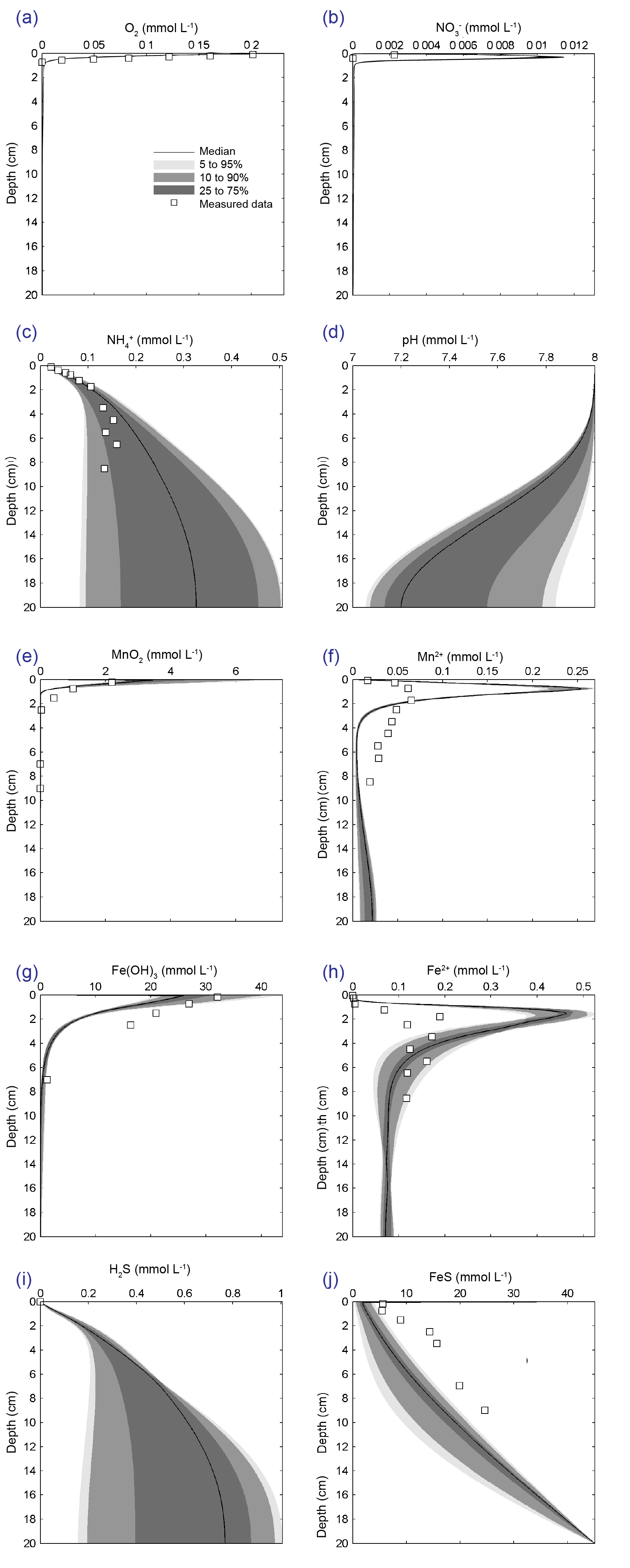
Concentration-depth profiles for major variables from 100 simulations, including the median result (black line), ranges of results (grey bands) and field data from Van Cappellen and Wang (1996) (squares).

Figure 14.53: Concentration-depth profiles for major variables from 100 simulations, including the median result (black line), ranges of results (grey bands) and field data from Van Cappellen and Wang (1996) (squares).

Reaction rates

The rates of aerobic respiration and denitrification using CANDI-AED were close to the simulated rates of Van Cappellen and Wang (1996), though in the deepest part of the sediment, the simulated aerobic rate was greater using this model (Figure 14.54 (b)). As a result of the classic inhibition sequence, oxygen penetration to greater depths limited denitrification to a deeper depth layer (Figure 14.54 (c)). This carried through to the peaks of all oxidation rates, which then occurred at slightly greater depths than in the Van Cappellen and Wang simulation. The maximum manganese reduction rate was smaller than in the Van Cappellen and Wang simulation, however, in both models the manganese reduction rate was very small relative to the other terminal oxidation processes (Figure 14.54 (d)). The iron reduction rate was similar to the Van Cappellen and Wang rate, although slightly smaller, and could not be increased without leading to greater discrepancy in the dissolved iron concentration profiles (Figure 14.54 (e)). The sulphate reduction profiles were very close and as with Van Cappellen and Wang, methanogenesis was completely inhibited (Figure 14.54 (f)).

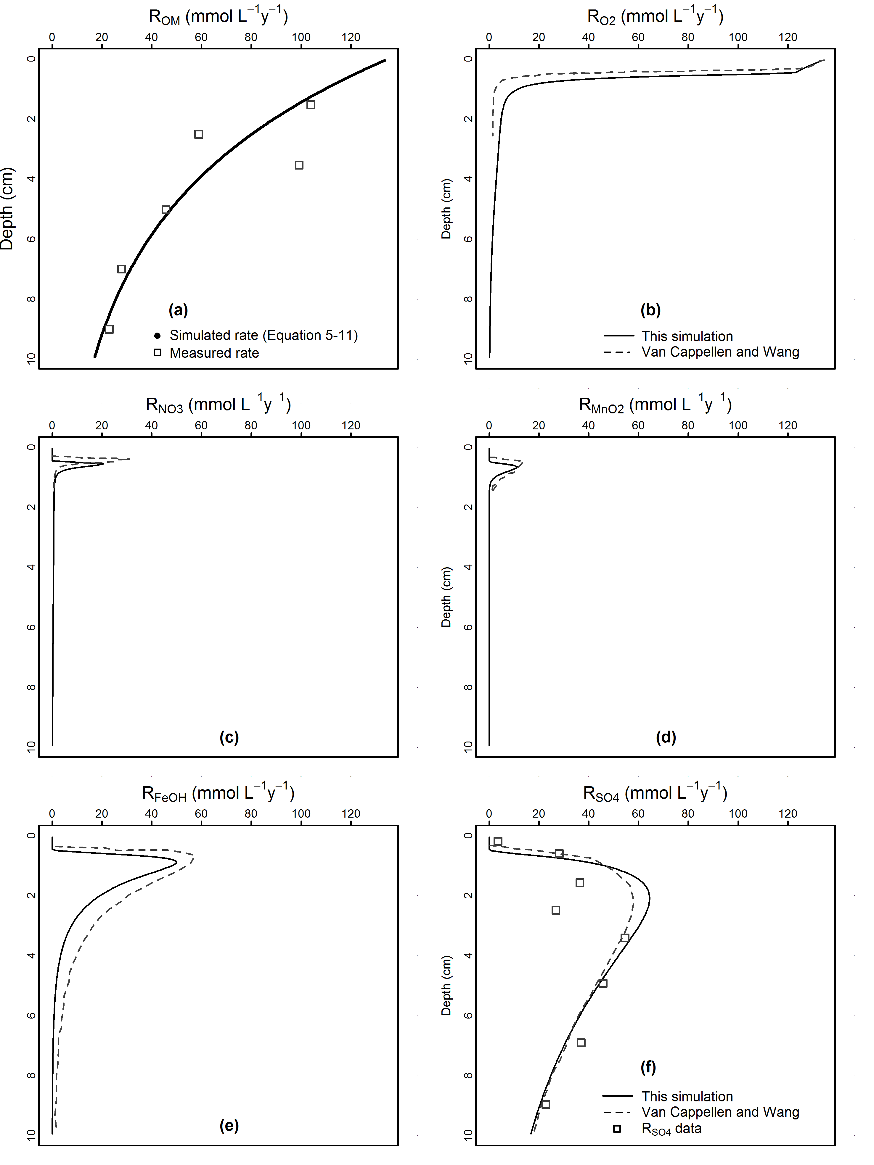
Figure 14.54: Profiles of organic matter oxidation rate with depth. Plot (a) was the total organic matter reaction rate set by a fixed depth-oxidation rate, which Van Cappellen and Wang based on the measured data (squares). Plots (b) to (f) are these simulated rates (solid lines) compared with the simulated rates of Van Cappellen and Wang (dashed lines) and in the case of sulphate reduction, measured data (squares, (f))

14.6.2 Case study: Aquaculture and sediment recovery

14.6.2.1 Introduction

This work was to calculate the potential effect of aquaculture on the sediment condition of fish cages propose for installation near Delma Island, UAE. The approach was similar to work done in 2015 on a proposed aquaculture site in the Abrolhos Islands, Western Australia (Paraska et al. 2015). The main objective of this part of the project was to calculate sediment chemical pore water concentrations and fluxes to the water column in response to variable deposition loads.

The primary input to the sediment model was reactive organic matter derived from aquaculture waste. This was calculated by models that tracked the transport and deposition of waste particles as a result of the hydrodynamics at the study site and different fish stocking scenarios. The organic matter deposition was then used as input to the sediment diagenesis model. The resulting waste particle distributions and sediment chemistry were then used to calculate the spatial effect of the cage operations on the sediment environment, as well as the greater chemistry and ecology of the water column.

The motivation behind the study was to ensure that potentially detrimental effects to the ecosystem were avoided. Fish cages may be positioned in one place for up to five years, after which the cage would be moved and the environment left to recover to its background condition (Figure 14.55).

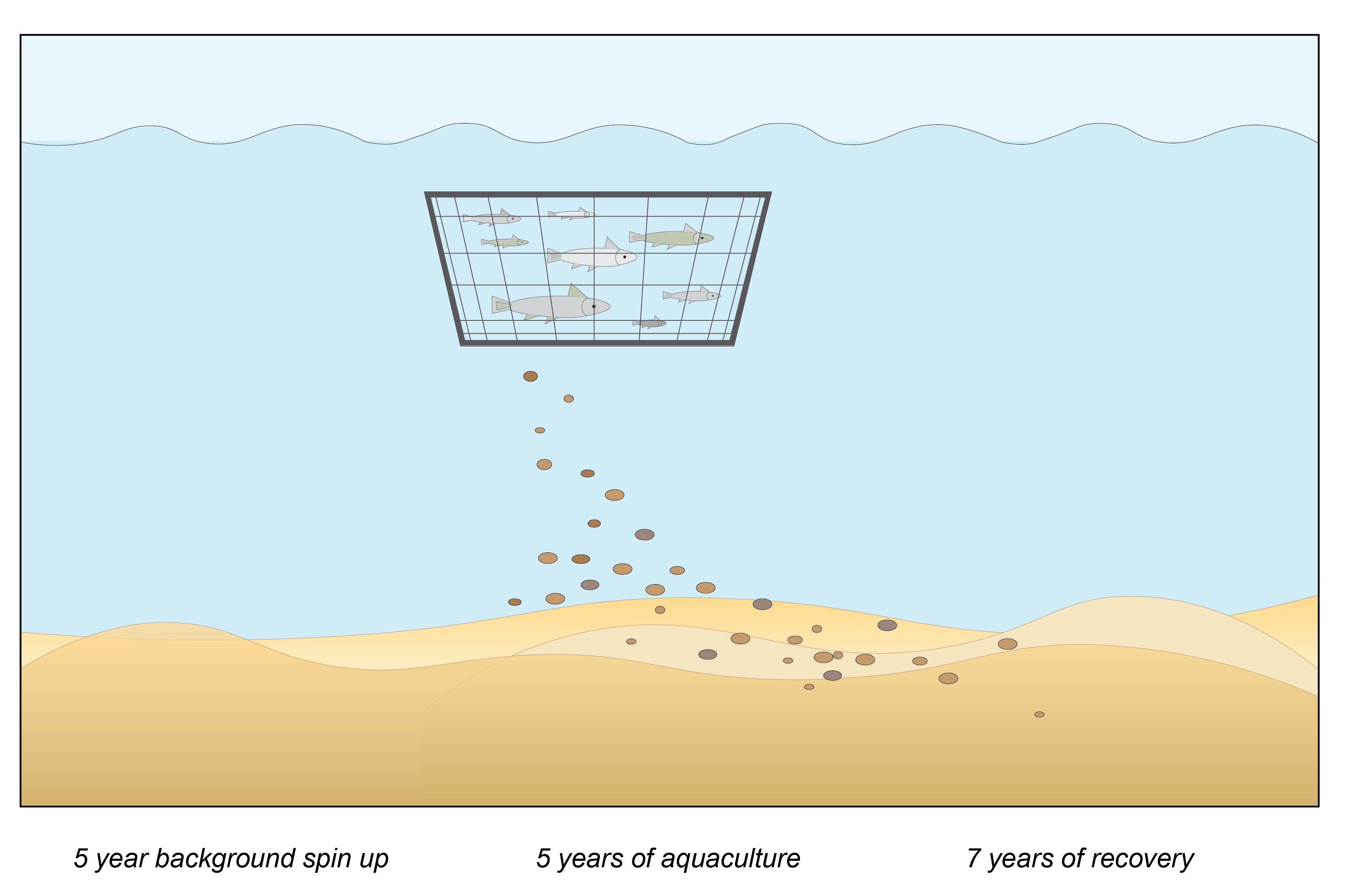
Schematic of the design of the aquaculture simulation. The simulation had a period of spin up, a period of aquaculture and then a recovery period.

Figure 14.55: Schematic of the design of the aquaculture simulation. The simulation had a period of spin up, a period of aquaculture and then a recovery period.

Given enough energy in the water column, the concentrations of chemicals can return to background relatively quickly. However, the conditions in the sediment can take much longer to recover to background levels, because the transport of chemicals is much slower. In particular, there may be a high concentration of $H_2S$ and low concentration of $O_2$, which together would make the environment uninhabitable for benthic fauna. Further, there may be an ongoing flux of nitrogen and phosphorus from the sediment to the water column, which could fuel algal blooms.

14.6.2.2 Methods

UAE study site chemical concentrations and fluxes

Field data was measured at the study site in October 2017 and analysed in November 2017. CANDI-AED was tailored to as many local conditions as possible. Since the $O_2$ and $NO_3^-$ concentrations were high and the $NH_4^+$ concentration was zero, it was assumed that the water column was aerobic. Total nitrogen in the sediment was measured as approximately 300 mg kg^-1, which was converted to approximately 30 mmol L^-1. Inorganic phosphate and total phosphate in the bottom water were set to zero, since their concentrations were below the detection limit. Total phosphorus in the sediment was measured as approximately 500 mg kg^-1, which was converted to approximately 20 mmol L^-1.

Total organic carbon was measured as approximately 0.6% carbon g sediment^-1. This was converted as approximately 600 mmol L^-1, after dividing by molecular mass and multiplying by bulk density. The C:N:P ratio of background organic matter fluxes was set after calibrating the top 5 cm of sediment to field conditions. This was calibrated well to field conditions, however, it resulted in a ratio that is rich in N and P compared to refractory carbon that is typically present in sediments. It was decided that given this uncertainty, it would be best to calibrate to field conditions. This also resulted in a conservative approach to calculating background nutrient fluxes, in that they would not be underestimated. $SO_4^{2-} concentration was set as the same for the bottom water boundary and for the initial sediment porewater concentration, since this was a marine site.

Manganese and iron concentrations were below the detection limit in the water column field data, and so they were set to zero in the simulations. The reaction of iron and manganese with organic matter can affect the generation of $H_2S$, and therefore the ecological effect on the surface sediments. Therefore, an extra simulation was run with assumed low background iron and manganese influxes, to examine the effect, as outlined below. Manganese and iron concentrations in the sediment were measurable, and so to reconcile this difference between sediment and water concentrations, it was assumed that the measured sediment iron and manganese reflected crystallized, non-reactive minerals (known in diagenesis models as $Fe(OH)_{3B}$ and $MnO_{2B}$).

Table 14.25: Details of water chemistry specification for the sediment model
Modelled variable	Field measurement (mg L^-1)	Modelled boundary (mmol L^-1)
O₂	7.60	2.4 x 102
NH₄⁺	0.00	0
NO₃^-	0.22	3.5 x 100
PO₄^3-	0.00	0
SO₄^2-	3163.00	3.3 x 104
Fe(OH)_3A	0.00	0
MnO_2A	0.00	0
HCO₃^-	109.00	1.8 x 103
CaCO₃	25.00	4.2 x 102
POM_R	1.86	1.6 x 102

Aquaculture waste input parameters

The C:N:P ratio of the aquaculture waste was supplied based on calculations based on a cage-model for fish biomass and waste properties. The rate constant for bacterial consumption of organic matter was set to 10 y^-1. This is one of the most uncertain, yet crucial parameters in diagenesis modelling. The equivalent value used by Brigolin et al (2009) was 8 y^-1. Considering that the water temperature at this study site may reach 40 °C, microbial metabolism, and therefore the rate constant, for all processes may approach a value twice as high as this. However, the value of 10 y^-1 was used in order to take a conservative approach to environmental recovery time.

Physical properties

The simulated sediment was 20 cm deep, and had 100 layers of exponentially increasing size from the sediment-water interface (0.25 mm) to the deepest layer (4 mm). The rate of particle deposition to the sediment-water interface was set to 0.2 cm y-1. Sediment porosity was not measured at the study site and so an assumption of 0.6 (water/total volume) was assumed for the bulk of the sediment, increasing to 0.9 in the upper 5 cm.

Simulation approach

The overall approach was to assess the sediment over a “gradient” of different waste loading intensities. The setup was a matrix of forty simulations, with ten input fluxes tested, each for 4 aquaculture durations (table 14.26).

Each simulation was for 23 years, with a 10 year period of background conditions, then the aquaculture period, then a recovery period. The duration of aquaculture was varied as either 1, 3 or 5 years. (For the larger fluxes, an additional period immediately following aquaculture was required, which had a fine time step.)

Table 14.26: Details of water chemistry specification for the sediment model
Modelled variable	Field measurement (mg L^-1)	Modelled boundary (mmol L^-1)
O₂	7.60	2.4 x 102
NH₄⁺	0.00	0
NO₃^-	0.22	3.5 x 100
PO₄^3-	0.00	0
SO₄^2-	3163.00	3.3 x 104
Fe(OH)_3A	0.00	0
MnO_2A	0.00	0
HCO₃^-	109.00	1.8 x 103
CaCO₃	25.00	4.2 x 102
POM_R	1.86	1.6 x 102

14.6.2.3 Results

Fluxes

Results of the steady state oxygen and nutrient fluxes being returned from the diagenesis model for the range of depositional rates (FOM) are shown below (figure 14.56, table 14.27.

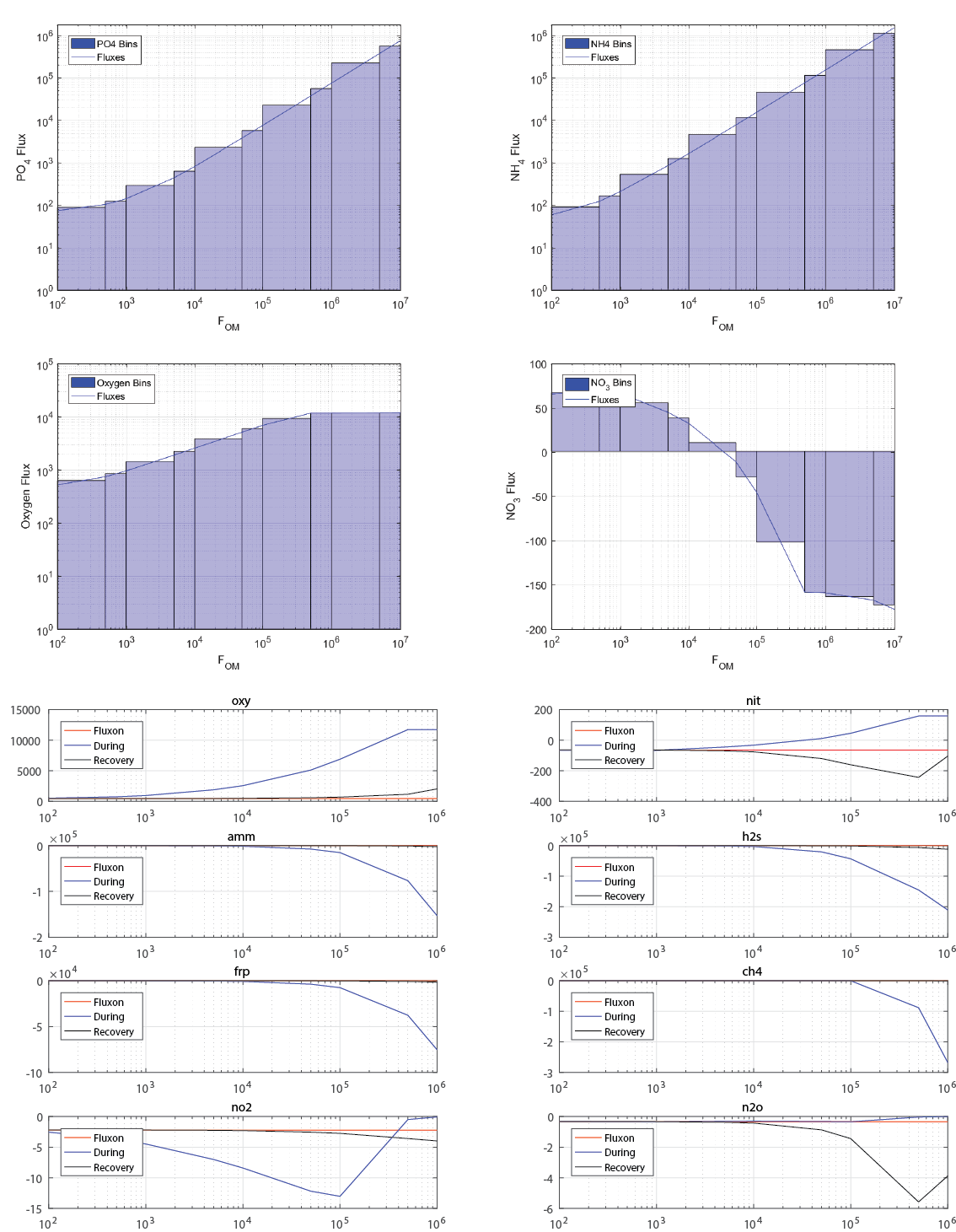
Figure 14.56: Summary of the nutrient fluxes at the sediment water interface returned from the diagenesis model for a wide range of input dpeositional flux rates.

Table 14.27: Nutrient and oxygen flux results for several depositional categories.
OM Flux upper range	NO₃^-	PO₄^3-	NH₄⁺	O₂
1×10⁷	178.0	-753000.0	-1.53e+06	12000
1×10⁷ to 5×10⁶	172.0	-564000.0	-1.15e+06	11900
5×10⁶ to 1×10⁶	163.0	-226000.0	-4.58e+05	11800
1×10⁶ to 5×10⁵	158.0	-56500.0	-1.15e+05	11700
5×10⁵ to 1×10⁵	102.0	-22600.0	-4.61e+04	9310
1×10⁵ to 5×10⁴	28.0	-5710.0	-1.17e+04	6000
5×10⁴ to 1×10⁴	-10.9	-2320.0	-4.73e+03	3840
1×10⁴ to 5×10³	-38.9	-628.0	-1.25e+03	2220
5×10³ to 1×10³	-56.1	-289.0	-5.28e+02	1410
1×10³ to 5×10²	-68.1	-120.0	-1.58e+02	827
5×10² to 1×10²	-66.9	-86.1	-8.35e+01	604
1×10²	-64.2	-70.9	-4.61e+01	460

Recovery time periods are shown below in Figure 14.57 UAEFish-3, and threshold depositional rates for recovery time categorisation is summarised in Table 14.28. The impact zone thresholds are summarised in Table 14.29.

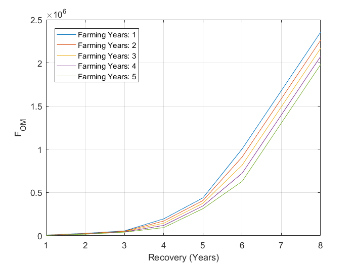
Predicted recovery time of the sediment for the 2cm oxygen and solfide concentration to return to within 85% of the pre-farmign value. Series depicted for aquaculture loading periods of 1-5 years.

Figure 14.57: Predicted recovery time of the sediment for the 2cm oxygen and solfide concentration to return to within 85% of the pre-farmign value. Series depicted for aquaculture loading periods of 1-5 years.

Table 14.28: Nutrient and oxygen flux results for several depositional categories.
Recovery time	1 Year	2 Years	3 Years	5 Years
<1 year recovery	0 to 202000	0 to 174000	0 to 145000	0 to 88100
2 year recovery	202000 to 480000	174000 to 403000	145000 to 327000	88100 to 173000
3 year recovery	480000 to 758000	403000 to 633000	327000 to 508000	173000 to 258000
4 year recovery	758000 to 1040000	633000 to 863000	508000 to 690000	258000 to 343000
5 year recovery	1040000 to 1310000	863000 to 1090000	690000 to 871000	343000 to 428000
6 year recovery	1310000 to 1590000	1090000 to 1320000	871000 to 1050000	428000 to 513000
7 year recovery	1590000 to 1870000	1320000 to 1550000	1050000 to 1230000	513000 to 598000
> 8 year recovery	1870000	1550000	1230000	598000

Table 14.29: Depositional thresholds for four impact zone settings, summarised for 4 aquaculture operation periods.
Zone	1 Year	2 Years	3 Years	5 Years
Zone of High Impact	78600	63000	47300	45100
Zone of Medium-High Impact	6300 to 78600	6200 to 63000	6100 to 47300	6000 to 45100
Zone of Medium Impact	1400 to 6300	1350 to 6200	1300 to 6100	1300 to 6000
Zone of Influence	1400	1350	1300	1300

14.6.3 Case study: The Coorong Dynamics Model

CANDI-AED was used as part of the assessment of the Coorong Lagoon in South Australia. It was used as part of a greater project, in conjunction with a fully 3D resolved Tuflow-FV model of the lagoon, that had full biogeochemistry modules and habitat assessments. In particular, the nutrient budgets and the effects of the hypersalinity were calculated. The sediment modelling component of the project in particular looked at the effect of hypersalinity on bioturbation and bioirrigation rates, and the resulting effects such as denitrification.

14.7 References

Berg, P., S. Rysgaard and B. Thamdrup (2003). Dynamic modeling of early diagenesis and nutrient cycling. A case study in an Arctic marine sediment. American Journal of Science 303(10): 905-955.

Berner, R. (1980). Early diagenesis: A theoretical approach. New Jersey, Princeton University Press.

Bethke, C., R. Sanford, M. Kirk, Q. Jin, and T. Flynn (2011), The thermodynamic ladder in geomicrobiology, American Journal of Science, 311(3): 183-210.

Boudreau, B. (1997). Diagenetic models and their implementation. Heidelberg, Springer.

Boudreau, B. and J. Westrich (1984). The dependence of bacterial sulfate reduction on sulfate concentration in marine sediments. Geochimica et Cosmochimica Acta 48(12): 2503-2516.

Boudreau, B. P. (1996). A method-of-lines code for carbon and nutrient diagenesis in aquatic sediments. Computers & Geosciences 22(5): 479-496.

Brigolin, D., R. Pastres, T. D. Nickell, C. J. Cromey, D. R. Aguilera and P. Regnier (2009). Modelling the impact of aquaculture on early diagenetic processes in sea loch sediments. Marine Ecology-Progress Series 388: 63-80.

Brown, P. N., G. D. Byrne, and A. C. Hindmarsh (1989), VODE: A variable-coefficient ODE solver, SIAM journal on scientific and statistical computing, 10(5): 1038-1051.

Dale, A. W., D. R. Aguilera, P. Regnier, H. Fossing, N. J. Knab and B. B. Jorgensen (2008a). Seasonal dynamics of the depth and rate of anaerobic oxidation of methane in Aarhus Bay (Denmark) sediments. Journal of Marine Research 66(1): 127-155.

Eldridge, P. and J. Morse (2008). Origins and temporal scales of hypoxia on the Louisiana shelf: Importance of benthic and sub-pycnocline water metabolism. Marine Chemistry 108(3-4): 159-171.

Fossing, H., P. Berg, B. Thamdrup, S. Rysgaard, H. Sorensen and K. Nielsen (2004). A model set-up for an oxygen and nutrient flux model for Aarhus Bay (Denmark).

Gaillard, J. F. and C. Rabouille (1992). Using Monod kinetics in geochemical models of organic carbon mineralisation in deep-sea surficial sediments. Deep-Sea Food Chains and the Global Carbon Cycle. G. T. Rowe and V. Pariente. 360: 309-324.

Jin, Q. S. and C. M. Bethke (2005). Predicting the rate of microbial respiration in geochemical environments. Geochimica et Cosmochimica Acta 69(5): 1133-1143.

Luff, R., K. Wallmann, S. Grandel and M. Schluter (2000). Numerical modeling of benthic processes in the deep Arabian Sea. Deep-sea research. Part 2, Topical studies in oceanography 47(14): 3039-3072.

Reed, D. C., C. P. Slomp and B. G. Gustafsson (2011b). Sedimentary phosphorus dynamics and the evolution of bottom-water hypoxia: A coupled benthic-pelagic model of a coastal system. Limnology and Oceanography 56(3): 1075-1092.

Soetaert, K., P. M. J. Herman and J. J. Middelburg (1996a). A model of early diagenetic processes from the shelf to abyssal depths. Geochimica et Cosmochimica Acta 60(6): 1019-1040.

Tufano, K. J., S. G. Benner, K. U. Mayer, M. A. Marcus, P. S. Nico, and S. Fendorf (2009), Aggregate-Scale Heterogeneity in Iron (Hydr)oxide Reductive Transformations All rights reserved. No part of this periodical may be reproduced or transmitted in any form or by any means, electronic or mechanical, including photocopying, recording, or any information storage and retrieval system, without permission in writing from the publisher, Vadose Zone J., 8(4): 1004-1012.

Van Cappellen, P. and Y. F. Wang (1996). Cycling of iron and manganese in surface sediments: A general theory for the coupled transport and reaction of carbon, oxygen, nitrogen, sulfur, iron, and manganese. American Journal of Science 296(3): 197-243.

–>

Approach	Limitation factor - FTEA	Inhibition factor - FIn
1	\(\displaystyle \ \frac {TEA}{TEA + K_{TEA} }\)	\(\displaystyle \ \frac {K_{In}} {TEA + K_{In} }\)
2	\(\displaystyle \ 0, \frac {TEA}{K_{TEA} } or 1\)	\(\displaystyle \ 1 - \frac {TEA}{K_{In} }\)

Description	Reaction	Rate equation
Simple NH₄⁺ oxidation by O₂	\(\displaystyle \ NH_4^++ 2O_2 + 2HCO_3^- \rightarrow NO_3^-+ 2CO_2 + 3H_2O\)	\(\displaystyle R_{NH4Ox} = k_{NH4Ox}[NH_4^+][O_2]\)
Ammonium oxidation	0	\(\displaystyle R_{Ammonium \ \ oxidation} = k_{NH4O2}[NH_4^+][O_2]\)
NH₄⁺ oxidation by O₂: nitrousation	\(\displaystyle \ 2NH_4^+ + 2O_2 + 2HCO_3^- \rightarrow N_2O + 2CO_2 + 5H_2O\)	\(\displaystyle R_{Nitrousation} = R_{Ammonium \ \ oxidation} \frac{K_{part \ \ ammox}}{K_{part\ \ ammox} + O_2}\)
NO₂^- oxidation by O₂: nitratation	\(\displaystyle \ NO_2^-+ \frac{1}{2} O_2 \rightarrow NO_3^-\)	\(\displaystyle R_{NO2O2} = k_{NO2O2}[NO_2^-][O_2]\)
NH₄⁺ oxidation by O₂: nitritation	\(\displaystyle \ NH_4^++ \frac{3}{2} O_2 + 2HCO_3^- \rightarrow NO_2^-+ 2CO_2 + 3H_2O\)	\(\displaystyle R_{NH4Ox} = R_{Ammonium \ \ oxidation} \frac{O_2}{K_{part \ \ ammox} + O_2}\)
NH₄⁺ oxidation by NO₂^- (Deammonification, anammox)	\(\displaystyle \ NH_4^+ + NO_2^- \rightarrow N_2 + 2H_2O\)	\(\displaystyle R_{NH4NO2} = k_{NH4NO2}[NH_4^+][O_2]\)
Mn²⁺ oxidation by O₂	\(\displaystyle \ Mn^{2+} + _{Xmk}X+ \frac{1}{2}O_2 + 2HCO_3^- \rightarrow MnO_{2A}-X_{Xmk}+ 2CO_2 + H_2O\)	\(\displaystyle R_{MnOx} = k_{MnOx}[Mn^{2+}][O_2]\)
Fe²⁺ oxidation by O₂	\(\displaystyle \ 4Fe^{2+}+ \frac{1}{2}O_2 + 4CO_2 + 2H_2O \rightarrow 4Fe^{3+}+ 4HCO_3^-\)	\(\displaystyle R_{FeOx} = k_{FeOx}[Fe^{2+}][O_2]\)
H₂S oxidation by O₂	\(\displaystyle \ H_2S+ 2O_2 + 2HCO_3^- \rightarrow SO_4^{2-}+ 2CO_2 + 2H_2O\)	\(\displaystyle R_{TSOx} = k_{TSOx}[H_2S][O_2]\)
CH₄ oxidation by O₂	\(\displaystyle \ CH_4+ O_2 \rightarrow + CO_2 + H_2O\)	\(\displaystyle R_{CH4Ox} = k_{CH4Ox}[CH_4][O_2]\)
FeS oxidation by O₂	\(\displaystyle \ FeS-X_{Xfm}+ O_2 \rightarrow SO_4^{2-} + Fe^{2+} + _{Xfm}X\)	\(\displaystyle R_{FeSOx} = k_{FeSOx}[FeS][O_2]\)
FeS₂ oxidation by O₂	\(\displaystyle \ FeS_2- X_{Xfm}+ 3.5O_2 + 2HCO_3^- \rightarrow Fe^{2+} + _{Xfm}X +2SO_4^{2-}+ 2CO_2 + H_2O\)	\(\displaystyle R_{FeS2Ox} = k_{FeS2Ox}[FeS_2][O_2]\)
Mn²⁺ oxidation by NO₃^-	\(\displaystyle \ 5Mn^{2+} + 2NO_3^- + 8HCO_3^- + _{xmk}X \rightarrow 5MnO_{2A}-_{xmk}X + 8CO_2 + 4H_2O + N_2\)	\(\displaystyle R_{MnNO3} = k_{MnNO3}[Mn^{2+}][NO_3^-]\)
Fe²⁺ oxidation by NO₃^-	\(\displaystyle \ 5Fe^{2+} + NO_3^-+ CO_2 + 3H_2O \rightarrow \frac{1}{2}N_2 + Fe^{3+} + 6HCO_3^-\)	\(\displaystyle R_{FeNO3} = k_{FeNO3}[Fe^{2+}][NO_3^-]\)
∑H₂S oxidation by NO₃^-	\(\displaystyle \ \frac{5}{2}H_2S + 4NO_3^- + HCO_3^- \rightarrow \frac{5}{2} SO_4^{2-} +2N_2 + CO_2 + 3H_2O\)	\(\displaystyle R_{TSNO3} = k_{TSNO3}[H_2S][NO_3^-]\)
Fe²⁺ oxidation by MnO_2A, _B	\(\displaystyle \ 2Fe^{2+} + 21X + (MnO_{2A}-X_{Xmk} + MnO_{2B}-X_{Xmk}) + 2HCO_3^- + 2H_2O \rightarrow 2Fe(OH)_{3A}-X_{xfl} + Mn^{2+} + kX + CO_2\)	\(\displaystyle R_{FeMn} = k_{FeMn}[Fe^{2+}][MnO_{2A, B}]\)
∑H₂S oxidation by MnO_2A, _B	\(\displaystyle \ H_2S + 4(MnO_{2A}-X_{Xmk} + MnO_{2A}-X_{Xmk}) + 6CO_2 + 2H_2O \rightarrow SO_4^{2-} + 4Mn^{2+}+ 4 _{Xmk}X + 6HCO_3^-\)	\(\displaystyle R_{TSMnO2} = k_{TSMnO2}[H_2S][MnO_{2A, B}]\)
FeS oxidation by MnO_2A, _B	\(\displaystyle \ FeS-X_{Xfm} + 4(MnO_{2A}-X_{Xmk} + MnO_{2B}-X_{Xmk} ) + 8CO_2 + 4H_2O \rightarrow SO_4^{2-} + 4Mn^{2+} + Fe^{2+} + (m + 4Xfm) X + 8HCO_3^-\)	\(\displaystyle R_{FeSMn} = k_{FeSMn}[FeS][MnO_{2A, B}]\)
∑H₂S oxidation by Fe(OH)_3A, _B	\(\displaystyle \ H_2S + 8(Fe(OH)_{3A}-X_{Xfl} + Fe(OH)_{3B}-X_{Xfl} ) + 14CO_2 \rightarrow SO_4^{2-} + 9 Fe^{2+} + 8_{XmK} X + 16HCO_3^- + 4H_2O\)	\(\displaystyle R_{TSFe} = k_{TSFe}[H_2S][Fe(OH)_{3A, B}]\)
FeS oxidation by Fe(OH)_3A, _B	\(\displaystyle \ FeS-X_{Xfl} + 8(Fe(OH)_{3A}-X_{Xfl} + Fe(OH)_{3A}-X_{Xfl}) + 16CO_2 \rightarrow SO_4^{2-} + 9 Fe^{2+} + (m+8Xfl)X + 16HCO_3^- + 4H_2O\)	\(\displaystyle R_{FeSFe} = k_{FeSFe}[FeS][Fe(OH)_{3A, B}]\)
CH₄ oxidation by SO₄^2-	\(\displaystyle \ CH_4 + SO_4^{2-} + CO_2 \rightarrow H_2S + 2HCO_3^-\)	\(\displaystyle R_{CH4SO4} = k_{CH4SO4}[CH_4][SO_2^{2-}]\)
H₂ oxidation by SO₄^2-	\(\displaystyle \ 5H_2 +SO_4^{2-} \rightarrow H_2S + 4H_2O\)	\(\displaystyle R_{HSO} = k_{HSO}[H_2][SO_4^{2-}]\)

Description	Reaction	Rate equation
Manganese
MnO₂ ageing	MnO_2A \(\rightarrow\) MnO_2B	If `rxn_mode` = 0 or 1, \(\displaystyle R_{MnO2Bppt} = 0\)

		If `rxn_mode` = 2, 3 or 4 \(\displaystyle \ \begin{align} R_{MnO2Bppt} = k_{MnO2Bppt} [MnO_{2B}] \end{align}\)
MnO_2A precipitation	2Mn²⁺ + O₂ + 4HCO₃^- \(\rightarrow\) 2MnO₂ + 4CO₂ +2H₂O	If `rxn_mode` = 0 or 1 \(\displaystyle \ R_{MnO2Appt} = 0\)

		If `rxn_mode` = 2 \(\displaystyle \ \begin{align} R_{MnO2Appt} = k_{MnO2Appt} [Mn^{2+}] \end{align}\)

		If `rxn_mode` = 3 \(\displaystyle \ \begin{align} \\ If IAP_{MnO2} = 0 \\ \\ R_{MnO2Appt} = k_{MnO2Appt} [Mn^{2+}] \\ \\ If IAP_{MnO2ppt} \lt 1 \\ \\ R_{MnO2Appt} = k_{MnO2Appt} (1 - (\frac {1 }{IAP_{MnO2} })) \\ \\ If IAP_{MnO2Appt} \ge 1 \\ \\ R_{MnO2Appt} = k_{MnO2Appt} (1 - (\frac {IAP_{MnO2} }{1 })) \end{align}\)

		If `rxn_mode` = 4 \(\displaystyle \ \begin{align} R_{MnO2Appt} = k_{MnO2Appt} [Mn^{2+}] \end{align}\)


Iron
Fe(OH)_3A ageing	4Fe(OH)_3A \(\rightarrow\) 4Fe(OH)_3B	If `rxn_mode` = 0 or 1, \(\displaystyle R_{FeOHBppt} = 0\)

		If `rxn_mode` = 2 \(\displaystyle \ \begin{align} R_{FeOHBppt} = k_{FeOHBppt} [Fe(OH)_{3B}] \end{align}\)

Fe(OH)_3A precipitation	4Fe²⁺ + O_2 + 8HCO_3^- + 2H_2O \(\rightarrow\) 4Fe(OH)3A + 8CO_2	If `rxn_mode` = 0 or 1, R_{FeOHAppt} = 0

		If `rxn_mode` = 2 \(\displaystyle \ \begin{align} R_{FeOHAppt} = k_{FeOHAppt} [Fe^{2+}] \end{align}\)

		If `rxn_mode` = 3 \(\displaystyle \ \begin{align} \\ If IAP_{FeOH} = 0 \\ \\ R_{FeOHAppt} = k_{FeOHAppt} [Fe^{2+}] \\ \\ If IAP_{FeOHA} \lt 1 \\ \\ R_{FeOHAppt} = k_{FeOHAppt} (1 - (\frac {1 }{IAP_{FeOH3} })) \\ \\ If IAP_{FeOH3} \ge 1 \\ \\ R_{FeOHAppt} = k_{FeOHAppt} (1 - (\frac {IAP_{FeOH3} }{1 })) \end{align}\)

		If `rxn_mode` = 4 \(\displaystyle \ \begin{align} R_{FeOHAppt} = k_{FeOHAppt} [Fe^{2+}] \end{align}\)

Description	Reaction	Rate equation
FeS transformation to FeS₂	FeS + H₂S \(\rightarrow\) FeS₂ + H₂	\(\displaystyle R_{Pyrite} = k_{Pyrite} [FeS][H_2S] \\ \)

FeS precipitation	Fe²⁺ + H₂S \(\rightarrow\) FeS + 2H⁺	If `rxn_mode` = 0 or 1 \(\displaystyle \ R_{FeS} = 0\)

		If `rxn_mode` = 2 \(\displaystyle \ R_{FeS} = k_{FeSppt}[Fe^2][HS^-]\)

		If `rxn_mode` = 3 \(\displaystyle \ \begin{align} R_{FeSppt} = k_{FeSppt}(1 - (\frac {K_{sp FeS} }{IAP_{FeS} })) \\ R_{FeSdiss} = - k_{FeSppt}(1 - (\frac {IAP_{FeS} } {K_{sp FeS} })) \end{align}\)

		If `rxn_mode` = 4 \(\displaystyle \ \begin{align} R_{FeSppt} = k_{FeSppt} \delta_{FeS} (\Omega_{FeS} - 1) \\ R_{FeSdiss} = k_{FeSdiss} \delta_{-FeS} (1 - \Omega_{FeS} ) \\ \Omega_{FeS} = (\frac {[Fe^{2+}]{HS^-} } {[H^+] K_{FeS}}) \\ If \Omega_{FeS} \gt 1 \ \delta_{FeS} = 1; \delta_{-FeS} = 0\ \\ If \Omega_{FeS} \le 1 \ \delta_{FeS} = 0; \delta_{-FeS} = 1 \end{align}\) \

Description	Reaction	Rate equation
MnCO₃
MnCO₃ precipitation	Mn²⁺ + CO₃^2- \(\rightarrow\) MnCO₃	If `rxn_mode` = 0 or 1 \(\displaystyle \ R_{Rodppt} = 0\)
		If `rxn_mode` = 2 \(\displaystyle \ R_{Rod} = k_{FeSppt} [Mn^{2+}] [HCO_3^-]\)

		If `rxn_mode` = 3 \(\displaystyle \ \begin{align} R_{Rodppt} = k_{Rodppt}(1 - (\frac {K_{sp Rod} }{IAP_{Rod} })) \\ R_{Roddiss} = - k_{Rodppt}(1 - (\frac {IAP_{Rod} } {K_{sp Rod} })) \end{align}\)

		If `rxn_mode` = 4 \(\displaystyle \ \begin{align} R_{Rodppt} = k_{Rodppt} \delta_{Rod} (\Omega_{Rod} - 1) \\ R_{Roddiss} = k_{Roddiss} \delta_{-Rod} (1 - \Omega_{Rod} ) \\ \Omega_{Rod} = (\frac {[Mn^{2+}]{CO_3^-} } { K_{Rod}}) \\ If \Omega_{Rod} \gt 1 \ \delta_{Rod} = 1; \delta_{-Rod} = 0\ \\ If \Omega_{Rod} \le 1 \ \delta_{Rod} = 0; \delta_{-Rod} = 1 \end{align}\)

FeCO₃
FeCO₃ precipitation	Fe²⁺ + CO₃^2- \(\rightarrow\) FeCO₃	If `rxn_mode` = 0 or 1 \(\displaystyle \ R_{Sidppt} = 0\)

		If `rxn_mode` = 2 \(\displaystyle \ R_{Sid} = k_{Sidppt} [Fe^{2+}] [HCO_3^-]\)

		If `rxn_mode` = 3 \(\displaystyle \ \begin{align} R_{Sidppt} = k_{Sidppt}(1 - (\frac {K_{sp Sid} }{IAP_{Sid} })) \\ R_{Siddiss} = - k_{Sidppt}(1 - (\frac {IAP_{Sid} } {K_{sp Sid} })) \end{align}\)

		If `rxn_mode` = 4 \(\displaystyle \begin{align} \ R_{Sidppt} = k_{Sidppt} \delta_{Sid} (\Omega_{Sid} - 1) \\ R_{Siddiss} = k_{Siddiss} \delta_{-Sid} (1 - \Omega_{Sid} ) \\ \Omega_{Sid} = (\frac {[Fe^{2+}]{CO_3^-} } { K_{Sid}}) \\ If \Omega_{Sid} \gt 1 \ \delta_{Sid} = 1; \delta_{-Sid} = 0\ \\ If \Omega_{Sid} \le 1 \ \delta_{Sid} = 0; \delta_{-Sid} = 1 \end{align}\)

CaCO₃
CaCO₃ precipitation	Ca²⁺ + CO₃^2- \(\rightarrow\) CaCO₃	If `rxn_mode` = 0 or 1 \(\displaystyle \ R_{Sidppt} = 0\)

		If `rxn_mode` = 2 \(\displaystyle \ R_{Cal} = k_{Calppt} [Ca^{2+}] [HCO_3^-]\)

		If `rxn_mode` = 3 \(\displaystyle \ \begin{align} R_{Calppt} = k_{Calppt}(1 - (\frac {K_{sp Cal} }{IAP_{Cal} })) \\ R_{Caldiss} = - k_{Calppt}(1 - (\frac {IAP_{Cal} } {K_{sp Cal} })) \end{align}\)

		If `rxn_mode` = 4 \(\displaystyle \ \begin{align} R_{Calppt} = k_{Calppt} \delta_{Cal} (\Omega_{Cal} - 1) \\ R_{Caldiss} = k_{Caldiss} \delta_{-Cal} (1 - \Omega_{Cal} ) \\ \Omega_{Cal} = (\frac {[Ca^{2+}]{CO_3^-} } { K_{Cal}}) \\ If \Omega_{Cal} \gt 1 \ \\ \delta_{Cal} = 1; \delta_{-Cal} = 0\ \\ If \Omega_{Cal} \le 1 \ \\ \delta_{Cal} = 0; \delta_{-Cal} = 1 \end{align}\)

Description	Reaction	Rate equation
OMModel 1
POM_Lab oxidation	POM_Lab \(\rightarrow\) CO₂ etc.	poml2dic ∑R_Oxi
POM_Ref oxidation	POM_Ref \(\rightarrow\) CO₂ etc.	pomr2dic ∑R_Oxi
POM_Ref oxidation	POM_Ref \(\rightarrow\) CO₂ etc.	pomspecial2dic ∑R_Oxi
OMModel2
POMLab hydrolysis	POM_Lab \(\rightarrow\) DOM_Lab	pocl2docl (POC_L)
POMRef hydrolysis	POMRef \(\rightarrow\) DOM_Ref	pocr2docr (POC_R)
DOMLab oxidation	DOMLab \(\rightarrow\) CO₂ etc.	docl2dic ∑R_Oxi
DOMRef oxidation	DOMRef \(\rightarrow\) CO₂ etc.	docr2dic ∑R_Oxi
OMModel 3
POMi hydrolysis	POMi \(\rightarrow\) D_Hyd	k~POM i~ (POM_i)F_BHyd
DHyd fermentation	DHyd \(\rightarrow\) OAc + H₂	k_growthB_FerF_T _FerF_DHyd
DHyd oxidation	DHyd \(\rightarrow\) CO₂ etc.	k_growthB_Aer,DenF_T _j F_DHyd
OAc, H2 oxidation	OAc, H2 \(\rightarrow\) CO₂ etc.	k_growthB_jF_T _j F_TEA _jF_OAc,H2 F_In _j
OMModel 4
POM oxidation	POM \(\rightarrow\) CO₂ etc.	R₀ e^(-\(\beta\) ^\(\times\) ^depth)

Description	.	Reaction
Denitrousation		\(\displaystyle \ (CH_2O)_x(NH_3)_y(PO_4)_z +2x N_2O + (-y + 2z) HCO_3^- \rightarrow 2xN_2 + (x-y+2z)CO_2 + (x-y+2z)H_2O + yNH_4^+ + zHPO_4^{3-}\)
Aerobic respiration		\(\displaystyle \ (CH_2O)_x(NH_3)_y(PO_4)_z +(x+2y)O_2 + (y + 2z) HCO_3^- \rightarrow + (x+y+2z)CO_2 + (x+y+2z)H_2O + yNH_4^+ + zHPO_4^{3-}\)
Denitritation		\(\displaystyle \ (CH_2O)_x(NH_3)_y(PO_4)_z +2x NO_3^- + (-y + 2z) HCO_3^- \rightarrow +2x NO_2^- + (x-y+2z)CO_2 + (x-y+2z)H_2O + yNH_4^+ + zHPO_4^{3-}\)
Nitrous denitritation		\(\displaystyle \ (CH_2O)_x(NH_3)_y(PO_4)_z + 2x NO-2^- + (-2x-y + 2z) HCO_3^- \rightarrow xN_2O + (x-y+2z)CO_2 + (-y+2z)H_2O + yNH_4^+ + zHPO_4^{3-}\)
DNRA		\(\displaystyle \ (CH_2O)_x(NH_3)_y(PO_4)_z + \frac{2x}{3}NO_2^- + (\frac{-4x}{3} -y +2z )HCO_3^-\rightarrow\\ \\ \frac{2x}{3} NH_4^+ (reduction \ \ product)+ (\frac{-x}{3}-y+2z)CO_2 + (-x-y+2z)H_2O + yNH_4^+ (from \ \ organic \ \ nitrogen) + zHPO_4^{3-}\)
Mn oxide reduction		\(\displaystyle \ (CH_2O)_x(NH_3)_y(PO_4)_z + 2xMnO_2 + (x + y - 2z) H_2O + (3x + y - 2z)CO_2 \rightarrow 2xMn^{2+} + (4x + y - 2z)HCO_3^- + yNH_4^+ + zHPO_4^{3-}\)
Fe oxide reduction		\(\displaystyle \ (CH_2O)_x(NH_3)_y(PO_4)_z + 4x FeOOH + (x + y - 2z) H_2O + (7x + y - 2z)CO_2 \rightarrow 4x Fe^{2+} + (8x + y - 2z)HCO_3^- + yNH_4^+ + zHPO_4^{3-}\)
Sulfate reduction		\(\displaystyle \ (CH_2O)_x(NH_3)_y(PO_4)_z + \frac{x}{2} SO_4^{2-} + (\frac{-x}{2} - y + 2z) HCO_3^- \rightarrow \frac{x}{2}HS^- + (\frac{x}{2} - y + 2z)CO_2 + (\frac{x}{2} - y + 2z)H_2O + yNH_4^+ + zHPO_4^{3-}\)
Methanogenesis		\(\displaystyle \ (CH_2O)_x(NH_3)_y(PO_4)_z + (- y + 2z) HCO_3^- \rightarrow 0.5 CH_4 + (0.5x - y + 2z)CO_2 + yNH_4^+ + zHPO_4^{3-}\)

Process	Rate equation
Denitratation	\(\displaystyle \ \ R_{Denitratation} = k_{OM} OM \frac {NO_3^-} {NO_3^- + K_{NO3} } \frac {K_{O2}^1} {O_2 + K_{O2}^1} \frac {K_{N2O}} {N_2O + K_{N2O}}\)
Denitritation	\(\displaystyle \ \ R_{Denitritation} = k_{OM} OM \frac {K_{O2}^3} {O_2 + K_{O2}^3 } \frac {K_{N2O}} {N_2O + K_{NO2} }\)
Nitrous denitritation	\(\displaystyle \ \ R_{Nitrous denitritation} = \frac {1} {2} R_{Denitritation} \frac {NO_2^- } {NO_2^- + K_{NO2} }\)
DNRA	\(\displaystyle \ \ R_{DNRA} = R_{Denitritation} \frac {K_{NO2} } {NO_2^- + K_{NO2} }\)
Denitrousation	\(\displaystyle \ \ R_{Denitrousation} = k_{OM} OM \frac {K_{N2O} } {K_{N2O}^6 +O_2 }\)
Ammonium release	\(\displaystyle \ \begin{align} \ R_{Ammonium release} = k_{OM} OM \times \\ (R_{Denitratation} + R_{Denitritation} + R_{Denitrousation}) \times \ \frac {N } {C } \end{align}\)

CANDI variable	Linked variable	Conversion	Description
PRES	id_depth	\(\displaystyle \times 1.025E-3\)	Pressure
TEMP	id_temp		Temperature
SALT	id_salt		Salinity
LGHT	id_par		Light
TAUB	id_taub		Diffusivity
MPBG	id_mpbg	\(\displaystyle \times \frac {1000 \times 365.25}{100 \times 100}\)	Microphytobenthos growth rate
MPBR	id_mpbr	\(\displaystyle \times \frac {1000 \times 365.25}{100 \times 100}\)	Microphytobenthos respiration rate
ROOT	id_rootb		Macrophyte root density
RTDP	id_rootd	\(\displaystyle \times \frac {1} {100}\)	Macrophyte root depth
RTO2	id_rooto	\(\displaystyle \times \frac {1000 \times 365.25}{100 \times 100}\)	Macrophyte root oxygen excretion

14 Sediment Biogeochemistry

14.1 Contributors

14.2 Overview

14.3 Model Description

14.3.1 General description

14.3.2 Process Descriptions

14.3.2.1 Sediment model domain

14.3.2.2 Physical Transport

Solids

Porewater

Porosity

14.3.2.3 Primary Redox Reactions

Organic matter pools and reactivity

C:N:P partitioning

The redox sequence

Limitation and inhibition factors

Nitrogen cycling

Calculation of the primary reactions

14.3.2.4 Secondary Redox Reactions

Calculation of the secondary reactions

14.3.2.5 Equilibrium Geochemistry

pH

Mineral precipitation and ageing

Adsorption

14.3.2.6 Biological dynamics

Benthic macrofauna

Bioturbation

Bioirrigation

Salinity inhibition

H2S inhibition

Benthic flora

Microphytobenthos

Aquatic macrophytes

14.3.3 Implementation within the AED framework

14.3.3.1 Sediment-water coupling

14.3.3.2 Resolving sediment zonation

14.3.3.3 Numerical solution

14.3.3.3.1 Solute transport equations: subroutine LiqMotion

14.3.3.3.1.1 The top layer of the array

14.3.3.3.1.2 The top layer of the sediment

14.3.3.3.1.3 All intermediate layers

14.3.3.3.1.4 The bottom-most layer

14.3.3.3.2 Solid transport equations: subroutine SolMotion

14.3.3.3.2.1 The top layer of the array

14.3.3.3.2.2 The top layer of the sediment

14.3.3.3.2.3 All intermediate layers

14.3.3.3.2.4 The bottom-most layer

14.3.3.4 Module program structure

14.3.4 Optional module links

14.3.5 Feedbacks to the host model

14.3.6 Variable summary

14.3.6.1 State variables

14.3.6.2 Diagnostic variables

14.3.6.3 Environmental variables

14.3.7 Parameter and option summary

14.3.7.1 Module settings: &aed_sed_candi

14.3.7.2 Zone-specific parameters

Physical domain and numerical parameters

Organic matter parameters

Secondary redox reactions

Geochemistry parameters

Hidden parameters: aed_readcandi.F90

14.4 Setup & Configuration

14.4.1 Setup details and examples

14.4.1.1 Hydrodynamic model setup details and examples

14.4.1.2 Module settings and examples

&aed_sed_candi

&aed_models

&aed_sedflux

&aed_sed_const2d

&aed_sediment

Fsed linking variables

14.4.1.3 Zone-specific parameter details and examples

Physical domain and numerical parameters

Organic matter parameters

Secondary redox parameters

Geochemistry parameters

14.4.1.4 Boundary setting details and examples

Sediment-water interface boundary

14.4.1.5 Initial condition setup details and examples

H₂S inhibition